Contents
TeX documents including PDF
Document files
Command for execution
Make png images from TeX pdf using ImageMagick command 'convert'
platex tex_fig_rotate.tex
dvipdfm tex_fig_rotate.dvi
convert -trim -density 400 tex_fig_rotate.pdf -bordercolor 'transparent' -border 20x20 -quality 100 fig_rotate.png

platex tex_flow.tex
dvipdfm tex_flow.dvi
convert -trim -density 400 tex_flow.pdf -bordercolor 'transparent' -border 20x20 -quality 100 fig_flow.png
Make main TeX pdf
platex en_theory.tex
dvipdfm en_theory.dvi
Interpolation Function and Gauss-Legendre Quadrature
Introduction
In the finite element method, it is necessary to express the physical quantities of any point in the element with nodal physical quantities using interpolation function $[\boldsymbol{N}]$.
For exmple, in the thermal conductivity analysis, a temperature at any point $T$ can be expressed as follow.
\begin{equation}
T=N_1(a,b)\cdot \phi_i+N_2(a,b)\cdot \phi_j+N_3(a,b)\cdot \phi_k+N_4(a,b)\cdot \phi_l
\end{equation}
where, $\phi_i$, $\phi_j$, $\phi_k$, $\phi_l$ mean the temperature at node $i$, $j$, $k$, $l$ for each.
If vectoe expression is applied,
\begin{equation}
T=\begin{bmatrix}N_1 & N_2 & N_3 & N_4 \end{bmatrix}\{\boldsymbol{\phi}\}=[\boldsymbol{N}]\{\boldsymbol{\phi}\}
\end{equation}
where, $\{\boldsymbol{\phi}\}$ means nodal temperature vector.
In this section, it is considered to use the Gauss-Legendre quadrature for 4 nodes element and to express the physical quantities using the normalized parameter coordinate $(a,b)$ with range of $[−1,1]$.
Interpolation function and its derivative
In actural calculation, since a mathematical expression and derivative of interpolation function are required, they will be derived.
After this, the interpolation function $N(a, b)$ is used, where $(a,b)$ is normalized parameter coordinate with range of $a=[−1,1]$ and $b=[−1,1]$.
Mathematical expression of interpolation function
For a 4 nodes element, following interpolation function can be applied.
\begin{align}
N_1=&\frac{1}{4}(1-a)(1-b) \qquad N_2=\frac{1}{4}(1+a)(1-b) \\
N_3=&\frac{1}{4}(1+a)(1+b) \qquad N_4=\frac{1}{4}(1-a)(1+b)
\end{align}
Derivative of interpolation function
The partial derivatives of $N$ about $a$ and $b$ can be obtained s follows.
\begin{align}
&\cfrac{\partial N_1}{\partial a}=-\cfrac{1}{4}(1-b) &\cfrac{\partial N_2}{\partial a}=+\cfrac{1}{4}(1-b) & &\cfrac{\partial N_3}{\partial a}=+\cfrac{1}{4}(1+b) & &\cfrac{\partial N_4}{\partial a}=-\cfrac{1}{4}(1+b) \\
&\cfrac{\partial N_1}{\partial b}=-\cfrac{1}{4}(1-a) &\cfrac{\partial N_2}{\partial b}=-\cfrac{1}{4}(1+a) & &\cfrac{\partial N_3}{\partial b}=+\cfrac{1}{4}(1+a) & &\cfrac{\partial N_4}{\partial b}=+\cfrac{1}{4}(1-a)
\end{align}
Next, above equations can be expressed using Jacobi matrix $[J]$ as follows.
\begin{equation}
\begin{Bmatrix} \cfrac{\partial N_i}{\partial a} \\ \cfrac{\partial N_i}{\partial b} \end{Bmatrix}
=[J] \begin{Bmatrix} \cfrac{\partial N_i}{\partial x} \\ \cfrac{\partial N_i}{\partial y} \end{Bmatrix} \qquad
\begin{Bmatrix} \cfrac{\partial N_i}{\partial x} \\ \cfrac{\partial N_i}{\partial y} \end{Bmatrix}
=[J]^{-1} \begin{Bmatrix} \cfrac{\partial N_i}{\partial a} \\ \cfrac{\partial N_i}{\partial b} \end{Bmatrix}
\end{equation}
\begin{equation}
[J]=\begin{bmatrix}
\cfrac{\partial x}{\partial a} & \cfrac{\partial y}{\partial a} \\
\cfrac{\partial x}{\partial b} & \cfrac{\partial y}{\partial b}
\end{bmatrix}
=\begin{bmatrix}
\displaystyle \sum_{i=1}^4\left(\cfrac{\partial N_i}{\partial a}x_i\right) & \displaystyle \sum_{i=1}^4\left(\cfrac{\partial N_i}{\partial a}y_i\right) \\
\displaystyle \sum_{i=1}^4\left(\cfrac{\partial N_i}{\partial b}x_i\right) & \displaystyle \sum_{i=1}^4\left(\cfrac{\partial N_i}{\partial b}y_i\right)
\end{bmatrix}
=\begin{bmatrix} J_{11} & J_{12} \\ J_{21} & J_{22} \end{bmatrix}
\end{equation}
\begin{equation}
[J]^{-1}=\frac{1}{\det(J)}\begin{bmatrix} J_{22} & -J_{12} \\ -J_{21} & J_{11} \end{bmatrix} \qquad
\det(J)=J_{11}\cdot J_{22}-J_{12}\cdot J_{21}
\end{equation}
From above,
\begin{equation}
\cfrac{\partial N_i}{\partial x}=\cfrac{1}{\det(J)}\left\{J_{22}\cfrac{\partial N_i}{\partial a}-J_{12}\cfrac{\partial N_i}{\partial b}\right\} \qquad
\cfrac{\partial N_i}{\partial y}=\cfrac{1}{\det(J)}\left\{-J_{21}\cfrac{\partial N_i}{\partial a}+J_{11}\cfrac{\partial N_i}{\partial b}\right\}
\end{equation}
the each element of $[J]$ can be shown as follows, where $x_{i,j,k,l}$ and $y_{i,j,k,l}$ means nodal coordinates which form a finite element.
\begin{align}
&J_{11}=\frac{\partial N_1}{\partial a} x_i+\frac{\partial N_2}{\partial a} x_j+\frac{\partial N_3}{\partial a} x_k+\frac{\partial N_4}{\partial a} x_l \\
&J_{12}=\frac{\partial N_1}{\partial a} y_i+\frac{\partial N_2}{\partial a} y_j+\frac{\partial N_3}{\partial a} y_k+\frac{\partial N_4}{\partial a} y_l \\
&J_{21}=\frac{\partial N_1}{\partial b} x_i+\frac{\partial N_2}{\partial b} x_j+\frac{\partial N_3}{\partial b} x_k+\frac{\partial N_4}{\partial b} x_l \\
&J_{22}=\frac{\partial N_1}{\partial b} y_i+\frac{\partial N_2}{\partial b} y_j+\frac{\partial N_3}{\partial b} y_k+\frac{\partial N_4}{\partial b} y_l
\end{align}
From above, the elements of $[J]$ were defined and derivative of $[\boldsymbol{N}]$ can be calculated.
At this point, it is necessary to note that $[J]$, $[\boldsymbol{N}]$ and its derivative are function of variables $a$ and $b$.
Gauss-Legendre quadrature
Gauss-Legendre quadrature is used for integration.
Surface integral
When 4 Gauss points ($n=2$) are considered in an finite element, the values of $a$, $b$ and weight $H$ can be shown in below table.
In this case, the approximation of integral value can be calculated as a summation of 4 times calculation depending on the coordinate $(a, b)$.
Furthermore, since the weight $H$ is equal to $1$ for all coordinate, the calculation can be more simplified.
\begin{equation}
\int_{-1}^{1}\int_{-1}^{1} f(a,b)\cdot da\cdot db
\doteqdot \sum_{i=1}^n\sum_{j=1}^n H_i\cdot H_j\cdot f(a_i,b_j)
= \sum_{kk=1}^4 f(a_{kk}, b_{kk})
\end{equation}
| i | j | a | b | H | kk |
|---|
| 1 | 1 | -0.57735 02692 | -0.57735 02692 | 1.00000 00000 | 1 |
| 1 | 2 | +0.57735 02692 | -0.57735 02692 | 1.00000 00000 | 2 |
| 2 | 1 | +0.57735 02692 | +0.57735 02692 | 1.00000 00000 | 3 |
| 2 | 2 | -0.57735 02692 | +0.57735 02692 | 1.00000 00000 | 4 |
Curvilinear integral
In the thermal conductivity analysis, curvilinear integral is requied on the element side which has heat transfer boundary condition.
The method of curvilinear integral along the element side is shown below.
| s1 | s2 | H |
|---|
| -0.57735 02692 | +0.57735 02692 | 1.00000 00000 |
General equilibrium equation for static structural analysis using principle of virtual work
In this section, a derivation of general equilibrium equation for static structural analysis using principle of virtual work is descrived.
Generally, in case that a elastic body subjected to the external force is under the equilibrium state, the virtual work due to the internal stresses in the body is equal to the virtual work due to the surface force or body force. This relationship can be expressed as follow.
\begin{equation}
\int_V \{\boldsymbol{\delta \epsilon}\}\{\boldsymbol{\sigma}\}dV=\int_A \{\boldsymbol{\delta u}\}\{\boldsymbol{S}\}dA+\int_V \{\boldsymbol{\delta u}\}\{\boldsymbol{F}\}dV
\end{equation}
| $\{\boldsymbol{\delta \epsilon}\}$ | : virtual strain in stress direction | $\{\boldsymbol{\sigma}\}$ | : internal stress in the doby |
| $\{\boldsymbol{\delta u}\}$ | : virtual displacement in force direction | $\{\boldsymbol{S}\}$ | : surface force |
| $V$ | : volume of a body | $\{\boldsymbol{F}\}$ | : body force (inertia force) |
| $A$ | : area of surface force acts | | |
At this point, it is assumed that a body deems an finite element and strain $\{\boldsymbol{\epsilon}\}$ and displacement $\{\boldsymbol{u}\}$ at any point in a fifite element can be expressed using nodal displacement $\{\boldsymbol{u}\}$ as follows.
\begin{align}
&\{\boldsymbol{\epsilon}\}=[\boldsymbol{B}]\{\boldsymbol{u_{nd}}\} \\
&\{\boldsymbol{u}\}=[\boldsymbol{N}]\{\boldsymbol{u_{nd}}\}
\end{align}
where, $[\boldsymbol{B}]$ is a strain-displacement relationship matrix, $[\boldsymbol{N}]$ is an interpolation function matrix.
And a stress-strain relationship of elastic body is applied shown below.
\begin{equation}
\{\boldsymbol{\sigma}\}=[\boldsymbol{D_e}]\{\boldsymbol{\epsilon}-\boldsymbol{\epsilon_0}\}
\end{equation}
where, $[\boldsymbol{D_e}]$ is stress-strain relationship matrix, $\{\boldsymbol{\epsilon_0}\}$ is initial strain due to temperature change and so on.
Next, it is assumed that $\{\boldsymbol{F}\}$ can be expressed using nodal inertia force $\{\boldsymbol{w_{nd}}\}$ as follow.
\begin{equation}
\{\boldsymbol{F}\}=[\boldsymbol{N}]\{\boldsymbol{w_{nd}}\}
\end{equation}
From above, left side of virtual work equation which means virtual work due to internal force becomes as follow.
\begin{align}
\int_V \{\boldsymbol{\delta \epsilon}\}\{\boldsymbol{\sigma}\}dV
=&\{\boldsymbol{\delta u_{nd}}\}^T \int_v[\boldsymbol{B}]^T\{\boldsymbol{\sigma}\}dV \\
=&\{\boldsymbol{\delta u_{nd}}\}^T \left(\int_V[\boldsymbol{B}]^T[\boldsymbol{D_e}][\boldsymbol{B}]dV\right) \{\boldsymbol{u_{nd}}\}
-\{\boldsymbol{\delta u_{nd}}\}^T \left(\int_V[\boldsymbol{B}]^T[\boldsymbol{D_e}]\{\boldsymbol{\epsilon_0}\}dV\right) \\
=&\{\boldsymbol{\delta u_{nd}}\}^T[\boldsymbol{k}]\{\boldsymbol{u_{nd}}\}-\{\boldsymbol{\delta u_{nd}}\}^T\{\boldsymbol{f_t}\}
\end{align}
And right side of virtual work equation which means virtual work due to external force becomes as follow.
\begin{align}
&\int_A \{\boldsymbol{\delta u}\}\{\boldsymbol{S}\}dA=\{\boldsymbol{\delta u_{nd}}\}^T \left(\int_A [\boldsymbol{N}]^T\{\boldsymbol{S}\}dA\right)=\{\boldsymbol{\delta u_{nd}}\}^T\{\boldsymbol{f}\} \\
&\int_V \{\boldsymbol{\delta u}\}\{\boldsymbol{F}\}dV=\{\boldsymbol{\delta u_{nd}}\}^T \left(\int_V [\boldsymbol{N}]^T [\boldsymbol{N}]dV\right)\{\boldsymbol{w_{nd}}\}=\{\boldsymbol{\delta u_{nd}}\}^T\{\boldsymbol{f_b}\}
\end{align}
As a result, general form of stiffness equation can be obtained shown below.
\begin{equation}
[\boldsymbol{k}]\{\boldsymbol{u_{nd}}\}=\{\boldsymbol{f}\}+\{\boldsymbol{f_t}\}+\{\boldsymbol{f_b}\}
\end{equation}
\begin{align}
&[\boldsymbol{k}]=\int_V[\boldsymbol{B}]^T[\boldsymbol{D_e}][\boldsymbol{B}]dV & & \text{(element stiffness matrix)}\\
&\{\boldsymbol{f}\}=\int_A [\boldsymbol{N}]^T\{\boldsymbol{S}\}dA & & \text{(nodal external force vector)}\\
&\{\boldsymbol{f_t}\}=\int_V[\boldsymbol{B}]^T[\boldsymbol{D_e}]\{\boldsymbol{\epsilon_0}\}dV & & \text{(nodal force vector due to initial strain)}\\
&\{\boldsymbol{f_b}\}=\left(\int_V [\boldsymbol{N}]^T [\boldsymbol{N}]dV\right)\{\boldsymbol{w_{nd}}\} & & \text{(nodal inertia force vector)}
\end{align}
Above equation is to calculate the displacement of the structure.
To calculate the stress of the element, following equation above mentioned shall be used.
\begin{equation}
\{\boldsymbol{\sigma}\}=[\boldsymbol{D_e}]\{\boldsymbol{\epsilon}-\boldsymbol{\epsilon_0}\}
\end{equation}
where, $\{\boldsymbol{\epsilon}\}$ means the strain vector of an element calculated from the displacements which are obtained by solving a stiffness equation.
2D Frame Analysis
Element stiffnes equation
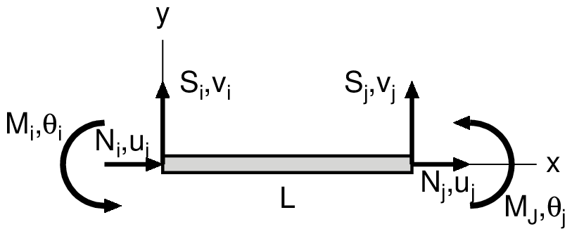
Element stiffness equation is shown below.
\begin{equation}
\{\boldsymbol{f}\}=[\boldsymbol{k}]\{\boldsymbol{u}\}
\end{equation}
\begin{equation}
\begin{Bmatrix} N_i \\ S_i \\ M_i \\ N_j \\ S_j \\ M_j \end{Bmatrix}
=\begin{bmatrix}
EA/L & 0 & 0 & -EA/L & 0 & 0 \\
0 & 12 EI/L^3 & 6 EI/L^2 & 0 & -12 EI/L^3 & 6 EI/L^2 \\
0 & 6 EI/L^2 & 4 EI/L & 0 & -6 EI/L^2 & 2 EI/L \\
-EA/L & 0 & 0 & EA/L & 0 & 0 \\
0 & -12 EI/L^3 & -6 EI/L^2 & 0 & 12 EI/L^3 & -6 EI/L^2 \\
0 & 6 EI/L^2 & 2 EI/L & 0 & -6 EI/L^2 & 4 EI/L
\end{bmatrix}
\begin{Bmatrix} u_i \\ v_i \\ \theta_i \\ u_j \\ v_j \\ \theta_j \end{Bmatrix}
\end{equation}
| $EA$ | axial rigidity | | $N$ | axial force | | $u$ | axial displacement (in x-direction) |
| $EI$ | bending rigidity | | $S$ | Shearing force | | $v$ | deflection (in y-direction) |
| $L$ | element length | | $M$ | bending moment | | $\theta$ | rotation |
 |
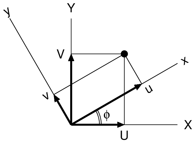 |
| Element displacements and forces | local coordinate system (x-y)
and global coordinate system (X-Y) |
|---|
Coordinate transformation matrix
Coordinate transformation matrix from global coordinate system to local coordinate system is shown below.
\begin{equation}
\{\boldsymbol{u}\}=[\boldsymbol{T}]\{\boldsymbol{U}\}
\end{equation}
\begin{equation}
\begin{Bmatrix} u_i \\ v_i \\ \theta_i \\ u_j \\ v_j \\ \theta_j \end{Bmatrix}
=
\begin{bmatrix}
\cos\phi & \sin\phi & 0 & 0 & 0 & 0 \\
-\sin\phi & \cos\phi & 0 & 0 & 0 & 0 \\
0 & 0 & 1 & 0 & 0 & 0 \\
0 & 0 & 0 & \cos\phi & \sin\phi & 0 \\
0 & 0 & 0 & -\sin\phi & \cos\phi & 0 \\
0 & 0 & 0 & 0 & 0 & 1
\end{bmatrix}
\begin{Bmatrix} U_i \\ V_i \\ \Theta_i \\ U_j \\ V_j \\ \Theta_j \end{Bmatrix}
\end{equation}
Stiffness equation in global coordinate system
Stiffness equation in global coordinate system is shown below. This shall be assemblied for all elements.
\begin{equation}
[\boldsymbol{K}]\{\boldsymbol{U}\}=\{\boldsymbol{F}\}+\{\boldsymbol{F_t}\}+\{\boldsymbol{F_b}\}
\end{equation}
| $[\boldsymbol{K}]=[\boldsymbol{T}]^T[\boldsymbol{k}][\boldsymbol{T}]$ | : stiffness matrix in global coordinate system |
| $\{\boldsymbol{U}\}$ | : nodal displacement vector in global coordinate system |
| $\{\boldsymbol{F}\}$ | : nodal external force vector in global coordinate system |
| $\{\boldsymbol{F_t}\}=[\boldsymbol{T}]^T\{\boldsymbol{f_t}\}$ | : nodal thermal load vector in global coordinate system |
| $\{\boldsymbol{F_b}\}=\{\boldsymbol{f_b}\}$ | : nodal inertia force vector in global coordinate system |
\begin{equation}
\{\boldsymbol{f_t}\}
=\begin{Bmatrix} -EA\cdot\alpha\cdot\Delta T \\ 0 \\ 0 \\ EA\cdot\alpha\cdot\Delta T \\ 0 \\ 0 \end{Bmatrix}
\qquad\qquad\qquad
\{\boldsymbol{f_b}\}
=\cfrac{\gamma A \ell}{2} \begin{Bmatrix} k_h \\ k_v \\ 0 \\ k_h \\ k_v \\ 0 \end{Bmatrix}
\end{equation}
| $EA$ | : axial rigidity | $\alpha$ | : thermal expansion coefficient | $\Delta T$ | : temperature change |
| $\gamma$ | : unit weight | $A$ | : element section area | $\ell$ | : element length |
| $k_h$ | : horiaontal acceleration | $k_v$ | : vertical acceleration | | |
Since element nodal thermal load vector $\{\boldsymbol{f_t}\}$ is a correction term of axial force of member, the coordinate transformation is requied when assemblied. Whereas, since element nodal inertia force vector $\{\boldsymbol{f_b}\}$ is defined using accelerations in global coordinate system, the coordinate transformation is not required when assemblied.
Furthermore, when section force is calculated from the solution of total stiffness equation, axial force shall be corrected as follows.
\begin{align}
N_{i}'=N_i+EA\cdot\alpha\cdot\Delta T \\
N_{j}'=N_j-EA\cdot\alpha\cdot\Delta T
\end{align}
2D Truss Analysis
Element stiffness equation
The element stiffness matrix of 2D truss consists of the matrix which doesn't include the item of rotation or moment of 2D frame element stiffness matrix.
The coordinate transformation matrix also doesn't include the item of rotation of that of 2D frame.
The element stiffness equation of 2D truss is shown below.
\begin{equation*}
\begin{Bmatrix} N_i \\ S_i \\ N_j \\ S_j \end{Bmatrix}
=\begin{bmatrix}
EA/L & 0 & -EA/L & 0 \\
0 & 0 & 0 & 0 \\
-EA/L & 0 & EA/L & 0 \\
0 & 0 & 0 & 0
\end{bmatrix}
\begin{Bmatrix} u_i \\ v_i \\ u_j \\ v_j \end{Bmatrix}
\end{equation*}
| $EA$ | axial rigidity | | $N$ | axial force | | $u$ | displacement in x-direction |
| $L$ | element length | | $S$ | shearing force | | $v$ | displacement in y-direction |
The coordinate transformation matrix of 2D truss is shown below.
\begin{equation}
\begin{Bmatrix} u_i \\ v_i \\ u_j \\ v_j \end{Bmatrix}
=
\begin{bmatrix}
\cos\phi & \sin\phi & 0 & 0 \\
-\sin\phi & \cos\phi & 0 & 0 \\
0 & 0 & \cos\phi & \sin\phi \\
0 & 0 & -\sin\phi & \cos\phi \\
\end{bmatrix}
\begin{Bmatrix} U_i \\ V_i \\ U_j \\ V_j \end{Bmatrix}
\end{equation}
Grid Girder Analysis
Element stiffness equation
The relationships of section forces between grid girder structure and 2D frame structure are shown below.
| Grid girder | 2D frame |
|---|
| Torsional moment | Axial force |
| Bending moment | Shearing force |
| Shearing force | Bending moment |
The element stiffness equation of grid girder structure is shown below.
\begin{equation*}
\begin{Bmatrix} T_i \\ M_i \\ Q_i \\ T_j \\ M_j \\ Q_j \end{Bmatrix}
=\begin{bmatrix}
GJ/L & 0 & 0 & -GJ/L & 0 & 0 \\
0 & 4 EI/L & -6 EI/L^2 & 0 & 2 EI/L & 6 EI/L^2 \\
0 & -6 EI/L^2 & 12 EI/L^3 & 0 & -6 EI/L^2 & -12 EI/L^3 \\
-GJ/L & 0 & 0 & GJ/L & 0 & 0 \\
0 & 2 EI/L & -6 EI/L^2 & 0 & 4 EI/L & 6 EI/L^2 \\
0 & 6 EI/L^2 & -12 EI/L^3 & 0 & 6 EI/L^2 & 12 EI/L^3
\end{bmatrix}
\begin{Bmatrix} \phi_i \\ \theta_i \\ w_i \\ \phi_j \\ \theta_j \\ w_j \end{Bmatrix}
\end{equation*}
| $GJ$ | tosional rigidity | | $T$ | tosional moment | | $\phi$ | rotation around x-axis |
| $EI$ | bending rigidity | | $M$ | bending moment | | $\theta$ | rotation around y-axis |
| $L$ | element length | | $Q$ | shearing force | | $w$ | deflection in z-direction |
Since the coordinate transformation is carried out on X-Y plane, the coordinate transformation matrix is the same as that for 2D frame analysis.
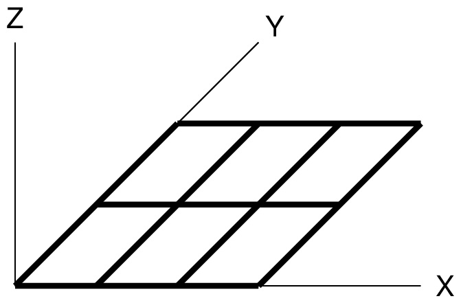 |
 |
| Global coordinate system | Local coordinate system |
|---|
(Reference) Torsional constant of rectangular cross section $J$
The torsional constant $J$ such as for concrete rectangular cross section can be calculated as follow.
\begin{equation}
J=\cfrac{h b^3}{3} \left\{1-\cfrac{192}{\pi^5} \cfrac{b}{h} \sum_{n=1}^\infty\left[\cfrac{1}{(2n-1)^5}\tanh\cfrac{(2n-1)\pi h}{2 b}\right]\right\} \qquad h \geqq b
\end{equation}
When the coefficient $\eta$ is introduced, the relationship between coefficient $\eta$ and the member dimension $h/b$ becomes shown below.
\begin{equation}
J=\cfrac{h b^3}{\eta}
\end{equation}
| $h/b$ | 1 | 2 | 3 | 5 | 10 | 20 |
|---|
| $\eta$ | 7.114 | 4.373 | 3.798 | 3.433 | 3.202 | 3.098 |
|---|
Above calculation was done by Python program shown below.
import numpy as np

### Result ###
# h/b  1.0    2.0    3.0    5.0    10.0   20.0
# eta  7.114  4.373  3.798  3.433  3.202  3.098
# J=h*b**3/eta

n=100
b=1.0
#hh=np.arange(1.0,21.0,1.0)
hh=np.array([1.0,2.0,3.0,5.0,10.0,20.0])
for idx,elem in enumerate(hh):
    h=elem
    s=0.0
    for i in range(1,n+1):
        s=s+1/(2*i-1)**5*np.tanh((2*i-1)*np.pi*h/2/b)
    x=1/3*(1-192/np.pi**5*b/h*s)
    print('{0:10.3f} {1:10.3f}'.format(h/b,1/x))
3D Frame Analysis
Element stiffness equation
\begin{equation*}
\boldsymbol{\{f\}}=\boldsymbol{[k]}\boldsymbol{\{u\}}
\end{equation*}
Nodal displacement vector
\begin{equation*}
\boldsymbol{\{u\}}=
\begin{Bmatrix}
u_i & v_i & w_i & \theta_{xi} & \theta_{yi} & \theta_{zi} & u_j & v_j & w_j & \theta_{xj} & \theta_{yj} & \theta_{zj}
\end{Bmatrix}^T
\end{equation*}
\begin{align*}
& u & \text{: displacement in x-direction} & & & \theta_x & \text{: rotation around x-axis} \\
& v & \text{: displacement in y-direction} & & & \theta_y & \text{: rotation around y-axis} \\
& w & \text{: displacement in z-direction} & & & \theta_z & \text{: rotation around z-axis}
\end{align*}
Nodal force vector
\begin{equation*}
\boldsymbol{\{f\}}=
\begin{Bmatrix}
N_i & S_{yi} & S_{zi} & M_{xi} & M_{yi} & M_{zi} & N_j & S_{yj} & S_{zj} & M_{xj} & M_{yj} & M_{zj}
\end{Bmatrix}^T
\end{equation*}
\begin{align*}
& N & \text{: axial force in x-direction} & & & M_x & \text{: moment around x-axis (tortional moment)} \\
& S_y & \text{: shear force in y-direction} & & & M_y & \text{: moment around y-axis (bending moment)} \\
& S_z & \text{: shear force in z-direction} & & & M_z & \text{: moment around z-axis (bending moment)}
\end{align*}
Element stiffness matrix
\begin{equation*}
\boldsymbol{[k]}=
\begin{bmatrix}
\cfrac{EA}{L} & 0 & 0 & 0 & 0 & 0 & -\cfrac{EA}{L} & 0 & 0 & 0 & 0 & 0 \\
0 & \cfrac{12EI_z}{L^3} & 0 & 0 & 0 & \cfrac{6EI_z}{L^2} & 0 & -\cfrac{12EI_z}{L^3} & 0 & 0 & 0 & \cfrac{6EI_z}{L^2} \\
0 & 0 & \cfrac{12EI_y}{L^3} & 0 & -\cfrac{6EI_y}{L^2} & 0 & 0 & 0 & -\cfrac{12EI_y}{L^3} & 0 & -\cfrac{6EI_y}{L^2} & 0 \\
0 & 0 & 0 & \cfrac{GJ}{L} & 0 & 0 & 0 & 0 & 0 & -\cfrac{GJ}{L} & 0 & 0 \\
0 & 0 & -\cfrac{6EI_y}{L^2} & 0 & \cfrac{4EI_y}{L} & 0 & 0 & 0 & \cfrac{6EI_y}{L^2} & 0 & \cfrac{2EI_y}{L} & 0 \\
0 & \cfrac{6EI_z}{L^2} & 0 & 0 & 0 & \cfrac{4EI_z}{L} & 0 & -\cfrac{6EI_z}{L^2} & 0 & 0 & 0 & \cfrac{2EI_z}{L} \\
-\cfrac{EA}{L} & 0 & 0 & 0 & 0 & 0 & \cfrac{EA}{L} & 0 & 0 & 0 & 0 & 0 \\
0 & -\cfrac{12EI_z}{L^3} & 0 & 0 & 0 & -\cfrac{6EI_z}{L^2} & 0 & \cfrac{12EI_z}{L^3} & 0 & 0 & 0 & -\cfrac{6EI_z}{L^2} \\
0 & 0 & -\cfrac{12EI_y}{L^3} & 0 & \cfrac{6EI_y}{L^2} & 0 & 0 & 0 & \cfrac{12EI_y}{L^3} & 0 & \cfrac{6EI_y}{L^2} & 0 \\
0 & 0 & 0 & -\cfrac{GJ}{L} & 0 & 0 & 0 & 0 & 0 & \cfrac{GJ}{L} & 0 & 0 \\
0 & 0 & -\cfrac{6EI_y}{L^2} & 0 & \cfrac{2EI_y}{L} & 0 & 0 & 0 & \cfrac{6EI_y}{L^2} & 0 & \cfrac{4EI_y}{L} & 0 \\
0 & \cfrac{6EI_z}{L^2} & 0 & 0 & 0 & \cfrac{2EI_z}{L} & 0 & -\cfrac{6EI_z}{L^2} & 0 & 0 & 0 & \cfrac{4EI_z}{L} \\
\end{bmatrix}
\end{equation*}
\begin{align*}
& L & \text{: element length} & & & & \\
& E & \text{: elastic modulus} & & & G & \text{: shear modulus} \\
& A & \text{: section area} & & & J & \text{: tortional constant} \\
& I_y & \text{: moment of inertia arounf y-axis} & & & I_z & \text{: moment of inertia around z-axis}
\end{align*}
Transformation matrix
Direction cosine of element axis (x-axis)
- An beam element has 2 nodes which are node-$i$ and node-$j$.
- The coordinate of node-$i$ is $(x_i,y_i,z_i)$, and the coordinate of node-$j$ is $(x_j,y_j,z_j)$.
- A direction cosine of an element axis which is the same as x-axis of an element can be expressed as following equations.
\begin{gather*}
l=\cfrac{x_j-x_i}{\ell} \qquad m=\cfrac{y_j-y_i}{\ell} \qquad n=\cfrac{z_j-z_i}{\ell} \\
\ell=\sqrt{(x_j-x_i)^2+(y_j-y_i)^2+(z_j-z_i)^2}
\end{gather*}
Submatrix of transformation matrix
$\boldsymbol{[t]}$ is a submatrix (3 x 3) of transformation matrix (12 x 12) which transforms the coordinate from global coordinate system to local coordinate system.
\begin{equation*}
\boldsymbol{\{x\}}=\boldsymbol{[t]}\boldsymbol{\{X\}}
\end{equation*}
where,
$\boldsymbol{\{x\}}$ means a vector in local coordinate system,
and $\boldsymbol{\{X\}}$ means a vector in global coordinate system.
(1) Case that x-axis in local coordinate system is not parallel to Z-axis in global coordinate system
\begin{equation*}
\boldsymbol{[t]}=
\begin{bmatrix}
1 & 0 & 0 \\
0 & \cos\theta & \sin\theta \\
0 & -\sin\theta & \cos\theta
\end{bmatrix}
\cdot
\begin{bmatrix}
l & m & n \\
-\cfrac{m}{\sqrt{l^2+m^2}} & \cfrac{l}{\sqrt{l^2+m^2}} & 0 \\
-\cfrac{l \cdot n}{\sqrt{l^2+m^2}} & -\cfrac{m \cdot n}{\sqrt{l^2+m^2}} & \sqrt{l^2+m^2}
\end{bmatrix}
\qquad \text{($\theta$ : chord angle)}
\end{equation*}
(2) Case that x-axis in local coordinate system is parallel to Z-axis in global coordinate system
In this case, since $x_j-x_i=0$,$y_j-y_i=0$ and $l=0$,$m=0$, it is necessary to re-write $\boldsymbol{[t]}$.
\begin{equation*}
\boldsymbol{[t]}=
\begin{bmatrix}
1 & 0 & 0 \\
0 & \cos\theta & \sin\theta \\
0 & -\sin\theta & \cos\theta
\end{bmatrix}
\cdot
\begin{bmatrix}
0 & 0 & n \\
n & 0 & 0 \\
0 & 1 & 0
\end{bmatrix}
\qquad \text{($\theta$ : chord angle)}
\end{equation*}
Full matrix of transformation matrix
\begin{equation*}
\boldsymbol{[T]}=
\begin{bmatrix}
\boldsymbol{[t]} & \boldsymbol{0} & \boldsymbol{0} & \boldsymbol{0} \\
\boldsymbol{0} & \boldsymbol{[t]} & \boldsymbol{0} & \boldsymbol{0} \\
\boldsymbol{0} & \boldsymbol{0} & \boldsymbol{[t]} & \boldsymbol{0} \\
\boldsymbol{0} & \boldsymbol{0} & \boldsymbol{0} &\boldsymbol{[t]}
\end{bmatrix}
\end{equation*}
Local coordinate system (x-y-z) with Zero chord angle in global coordinate system (X-Y-Z)
2D Stress Analysis
Finite element equation formulation
Calculation formula for nodal displacements
\begin{equation}
[\boldsymbol{k}]\{\boldsymbol{u}\}=\{\boldsymbol{f}\}+\{\boldsymbol{f_t}\}+\{\boldsymbol{f_b}\}
\end{equation}
\begin{align}
&[\boldsymbol{k}]=t\cdot \int_A [\boldsymbol{B}]^T[\boldsymbol{D}][\boldsymbol{B}] dA \\
&\{\boldsymbol{f_t}\}=t\cdot \int_A [\boldsymbol{B}]^T[\boldsymbol{D}]\{\boldsymbol{\epsilon_0}\} dA \\
&\{\boldsymbol{f_b}\}=t\cdot\gamma\cdot \int_A [\boldsymbol{N}]^T [\boldsymbol{N}] dA \cdot \{\boldsymbol{w}\}
\end{align}
Calculation formula for element stresses
\begin{equation}
\{\boldsymbol{\sigma}\}=[\boldsymbol{D}]\{\boldsymbol{\epsilon}-\boldsymbol{\epsilon_0}\}
\end{equation}
In the calculation formula for nodal displacements, the thermal load vector $\{\boldsymbol{f_t}\}$ is included in the items of load vector. However, in the element stresses calculation, the initial strain due to temperature change shall be subtracted from the strain which are calculated from the nodal displacements shown in above formula.
Equation of relationship between nodal displacement and strain at any points
\begin{equation}
\{\boldsymbol{\epsilon}\}=[\boldsymbol{B}]\{\boldsymbol{u}\}
\end{equation}
Equation of nodal displacement and displacement at any point
\begin{equation}
\{\boldsymbol{v}\}=[\boldsymbol{N}]\{\boldsymbol{u}\}
\end{equation}
| $[\boldsymbol{k}]$ | : element stiffness matrix |
| $\{\boldsymbol{u}\}$ | : nodal displacement vector |
| $\{\boldsymbol{f}\}$ | : nodal external force vector |
| $\{\boldsymbol{f_t}\}$ | : nodal load vector due to temperature change |
| $\{\boldsymbol{f_b}\}$ | : nodal body force vector |
| $[\boldsymbol{D}]$ | : stress-strain relationship matrix |
| $t$, $\gamma$ | : element thickness, element unit weight |
| $\{\boldsymbol{w}\}$ | : nodal acceleration vector (ratio to 'g') |
| $\{\boldsymbol{\epsilon_0}\}$ | : elemen strain due to temperature change |
| $\{\boldsymbol{\epsilon}\}$ | : element strain at any point |
| $\{\boldsymbol{v}\}$ | : element displacement at any point |
Stress-strain relationship on 2D elastic problem
AS well known as Hooke's law, stress-strain relationship for 3D isotropic elastic body can be expressed as follow, where $E$ is elastic modulus, $\nu$ is Poisson's ratio, $\alpha$ is thermal expansion coefficient, $T$ is temperature change.
\begin{equation}
\epsilon_x-\alpha T=\cfrac{1}{E}[\sigma_x-\nu(\sigma_y+\sigma_z)] \qquad
\epsilon_y-\alpha T=\cfrac{1}{E}[\sigma_y-\nu(\sigma_z+\sigma_x)] \qquad
\epsilon_z-\alpha T=\cfrac{1}{E}[\sigma_z-\nu(\sigma_x+\sigma_y)]
\end{equation}
\begin{equation}
\gamma_{xy}=\cfrac{2(1+\nu)}{E}\tau_{xy} \qquad
\gamma_{yz}=\cfrac{2(1+\nu)}{E}\tau_{yz} \qquad
\gamma_{zx}=\cfrac{2(1+\nu)}{E}\tau_{zx}
\end{equation}
When considering $x-y$ plane, in the plane stress state,
\begin{equation}
\sigma_z=0 \qquad \tau_{yz}=0 \qquad \tau_{zx}=0
\end{equation}
Therefore,
\begin{gather}
\epsilon_x-\alpha T=\cfrac{1}{E}(\sigma_x-\nu\sigma_y) \qquad
\epsilon_y-\alpha T=\cfrac{1}{E}(\sigma_y-\nu\sigma_x) \qquad
\gamma_{xy}=\cfrac{2(1+\nu)}{E}\tau_{xy} \\
\Longrightarrow
\begin{Bmatrix} \sigma_x \\ \sigma_y \\ \tau_{xy} \end{Bmatrix}
=\frac{E}{1-\nu^2}\begin{bmatrix} 1 & \nu & 0 \\ \nu & 1 & 0 \\ 0 & 0 & \cfrac{1-\nu}{2} \end{bmatrix}
\begin{Bmatrix} \epsilon_x-\alpha T \\ \epsilon_y-\alpha T \\ \gamma_{xy} \end{Bmatrix}
\end{gather}
In the plane strain state,
\begin{equation}
\epsilon_z=0 \rightarrow \sigma_z=\nu(\sigma_x+\sigma_y)-E\alpha T \qquad \tau_{yz}=0 \qquad \tau_{zx}=0
\end{equation}
Therefore,
\begin{gather}
\epsilon_x-\alpha T=\cfrac{1}{E}[(1-\nu^2)\sigma_x-\nu(1+\nu)\sigma_y] \qquad
\epsilon_y-\alpha T=\cfrac{1}{E}[(1-\nu^2)\sigma_y-\nu(1+\nu)\sigma_x] \qquad
\gamma_{xy}=\cfrac{2(1+\nu)}{E}\tau_{xy} \\
\Longrightarrow
\begin{Bmatrix} \sigma_x \\ \sigma_y \\ \tau_{xy} \end{Bmatrix}
=\frac{E}{(1+\nu)(1-2\nu)}\begin{bmatrix} 1-\nu & \nu & 0 \\ \nu & 1-\nu & 0 \\ 0 & 0 & \cfrac{1-2\nu}{2} \end{bmatrix}
\begin{Bmatrix} \epsilon_x-(1+\nu)\alpha T \\ \epsilon_y-(1+\nu)\alpha T \\ \gamma_{xy} \end{Bmatrix}
\end{gather}
The rearranged result of above can be shown as follows.
Stress and strain components in 2D elastic problem
\begin{equation}
\text{Stress component: }\{\boldsymbol{\sigma}\}=\begin{Bmatrix} \sigma_{x} \\ \sigma_{y} \\ \tau_{xy} \end{Bmatrix} \qquad
\text{Strain component: }\{\boldsymbol{\epsilon}\}=\begin{Bmatrix} \epsilon_{x} \\ \epsilon_{y} \\ \gamma_{xy} \end{Bmatrix}
\end{equation}
\begin{align}
&\text{Thermal strain component in plane stress state: }\{\boldsymbol{\epsilon_0}\}=\begin{Bmatrix} \alpha T \\ \alpha T \\ 0 \end{Bmatrix} \\
&\text{Thermal strain component in plane strain state: }\{\boldsymbol{\epsilon_0}\}=\begin{Bmatrix} (1+\nu)\alpha T \\ (1+\nu)\alpha T \\ 0 \end{Bmatrix}
\end{align}
where, tensile stress and tensile strain have positive sign, and temperature increase has positive sign.
Stress-strain relationship in 2D elastic problem
\begin{equation}
\text{Plane stress state: }[\boldsymbol{D_e}]=\frac{E}{1-\nu^2}\begin{bmatrix} 1 & \nu & 0 \\ \nu & 1 & 0 \\ 0 & 0 & \cfrac{1-\nu}{2} \end{bmatrix} \qquad
\begin{matrix} E & \text{: elastic modulus} \\ \nu & \text{: Poisson's ratio} \end{matrix}
\end{equation}
\begin{equation}
\text{Plane strain state: }[\boldsymbol{D_e}]=\frac{E}{(1+\nu)(1-2\nu)}\begin{bmatrix} 1-\nu & \nu & 0 \\ \nu & 1-\nu & 0 \\ 0 & 0 & \cfrac{1-2\nu}{2} \end{bmatrix}
\end{equation}
Formulation as isoparametric element with 4 nodes 4 Gouss points
Introduction of strain-nodal displacement relationship matrix $[\boldsymbol{B}]$
The displacements $u$,$v$ at any point in a quadrilateral element are assumed as follows, where coordinate ($a$,$b$) is normalized parameter coordinate with range of [$-1$,$1$] for each of $a$ or $b$, $u_{i,j,k,l}$ and $v_{i,j,k,l}$ are nodal displacements which forms an element.
\begin{align}
u=&N_1(a,b)\cdot u_i+N_2(a,b)\cdot u_j+N_3(a,b)\cdot u_k+N_4(a,b)\cdot u_l \\
v=&N_1(a,b)\cdot v_i+N_2(a,b)\cdot v_j+N_3(a,b)\cdot v_k+N_4(a,b)\cdot v_l
\end{align}
When the displacements at any point in an element is defined as $\{\boldsymbol{u}\}$, and the nodal displacements is defined as $\{\boldsymbol{u_{nd}}\}$, following expression can be obtained using matrix expression.
\begin{equation}
\{\boldsymbol{u}\}=\begin{Bmatrix} u \\ v \end{Bmatrix}
=\begin{bmatrix}
N_1 & 0 & N_2 & 0 & N_3 & 0 & N_4 & 0 \\
0 & N_1 & 0 & N_2 & 0 & N_3 & 0 & N_4
\end{bmatrix}
\begin{Bmatrix}
u_i \\ v_i \\ u_j \\ v_j \\ u_k \\ v_k \\ u_l \\ v_l
\end{Bmatrix}
=[\boldsymbol{N}]\{\boldsymbol{u_{nd}}\}
\end{equation}
The strainat any point in an element $\{\boldsymbol{\epsilon}\}$ can be expressed using nodal displacement $\{\boldsymbol{u_{nd}}\}$.
\begin{equation}
\{\boldsymbol{\epsilon}\}=\begin{Bmatrix} \cfrac{\partial u}{\partial x} \\ \cfrac{\partial v}{\partial y} \\ \cfrac{\partial u}{\partial y}+\cfrac{\partial v}{\partial x} \end{Bmatrix}
=\begin{bmatrix}
\cfrac{\partial N_1}{\partial x} & 0 & \cfrac{\partial N_2}{\partial x} & 0 & \cfrac{\partial N_3}{\partial x} & 0 & \cfrac{\partial N_4}{\partial x} & 0 \\
0 & \cfrac{\partial N_1}{\partial y} & 0 & \cfrac{\partial N_2}{\partial y} & 0 & \cfrac{\partial N_3}{\partial y} & 0 & \cfrac{\partial N_4}{\partial y} \\
\cfrac{\partial N_1}{\partial y} & \cfrac{\partial N_1}{\partial x} & \cfrac{\partial N_2}{\partial y} & \cfrac{\partial N_2}{\partial x} & \cfrac{\partial N_3}{\partial y} & \cfrac{\partial N_3}{\partial x} & \cfrac{\partial N_4}{\partial y} & \cfrac{\partial N_4}{\partial x}
\end{bmatrix}
\begin{Bmatrix}
u_i \\ v_i \\ u_j \\ v_j \\ u_k \\ v_k \\ u_l \\ v_l
\end{Bmatrix}
=[\boldsymbol{B}]\{\boldsymbol{u_{nd}}\}
\end{equation}
Element stiffness matrix
A stiffness matrix of 4 nodes isoparametric element $[\boldsymbol{k}]$ can be expressed as follow using the constant element thickness $t$ and stress-strain relationship matrix $[\boldsymbol{D_e}]$.
\begin{equation}
[\boldsymbol{k}]=t\int_{-1}^{1}\int_{-1}^{1}[\boldsymbol{B}]^{T}[\boldsymbol{D_e}][\boldsymbol{B}]\cdot\det(J)\cdot da\cdot db
=t\cdot \sum_{kk=1}^4 \left\{[\boldsymbol{B}]^{T}[\boldsymbol{D_e}][\boldsymbol{B}]\cdot\det(J)\right\}_{kk}
\end{equation}
Nodal force vector due to temperature change
Nodal force vector {\boldsymbol{f_t}\}$ due to thermal strain$\{\boldsymbol{\epsilon_0}\}$ can be expressed as follow.
\begin{equation}
\{\boldsymbol{f_t}\}=t\int_{-1}^{1}\int_{-1}^{1}[\boldsymbol{B}]^{T}[\boldsymbol{D_e}]\{\boldsymbol{\epsilon_0}\}\cdot\det(J)\cdot da\cdot db
=t\cdot \sum_{kk=1}^4 \left\{[\boldsymbol{B}]^{T}[\boldsymbol{D_e}]\{\boldsymbol{\epsilon_0}\}\cdot\det(J)\right\}_{kk}
\end{equation}
The component of strain due to temperature change is shown below.
\begin{equation}
T_p=N_1\cdot\phi_i+N_2\cdot\phi_j+N_3\cdot\phi_k+N_4\cdot\phi_l
\end{equation}
\begin{align}
\text{Plane stress srate: }&\{\boldsymbol{\epsilon_0}\}=\begin{Bmatrix} \alpha T_p \\ \alpha T_p \\ 0 \end{Bmatrix}
\\
\text{Plane strain state: }&\{\boldsymbol{\epsilon_0}\}=\begin{Bmatrix} (1+\nu)\alpha T_p \\ (1+\nu)\alpha T_p \\ 0 \end{Bmatrix}
\end{align}
where, $\alpha$ is thermal expansion coefficient, $\nu$ is Poisson's ratio, $T_p$ is temperature change at any point in an element, $\{\phi_i~~\phi_j~~\phi_k~~\phi_l\}^T$ is nodal temperature change vector, $[N_1~~N_2~~N_3~~N_4]$ is elements of interpolation function $[\boldsymbol{N}]$. And temperature increase has positive sign.
Nodal force vector due to body force
Body force (inertia force) at any point in a element $\{\boldsymbol{F}\}=\{F_{Bx},F_{By}\}^T$ can be expressed using nodal force vector $\{w\}$ and interpolation function$[\boldsymbol{N}]$.
\begin{equation}
\{\boldsymbol{F}\}=[\boldsymbol{N}]\{\boldsymbol{w}\}
\end{equation}
\begin{equation}
[\boldsymbol{N}]=\begin{bmatrix}N_1 & 0 & N_2 & 0 & N_3 & 0 & N_4 & 0\\ 0 & N_1 & 0 & N_2 & 0 & N_3 & 0 & N_4\end{bmatrix}
\end{equation}
\begin{equation}
\{\boldsymbol{w}\}=\gamma\cdot\begin{Bmatrix}k_h & k_v & k_h & k_v & k_h & k_v & k_h & k_v \end{Bmatrix}^T
\end{equation}
where, $\gamma$ is element unit weight (mass $\times$ gravity acceleration), $k_h$ and $k_v$ are horiaontal and vertical acceleration (ratio to 'g').
From above, nodal force vector due to body force (inertia force) $\{\boldsymbol{f_b}\}$ becomes can be calculated as follow.
\begin{equation}
\{\boldsymbol{f_b}\}=t\cdot\int_{A}[\boldsymbol{N}]^T\{\boldsymbol{F}\}dA
=t\cdot\gamma\cdot\int_{A}[\boldsymbol{N}]^T[\boldsymbol{N}]dA\cdot\{\boldsymbol{w'}\}
=t\cdot\gamma\cdot\sum_{kk=1}^4 \left\{[\boldsymbol{N}]^T[\boldsymbol{N}]\cdot\det(J)\right\}_{kk}\cdot\{\boldsymbol{w'}\}
\end{equation}
The vector $\{\boldsymbol{w}\}$ is defined as follow by pulling out $\gamma$.
\begin{equation}
\{\boldsymbol{w'}\}=\begin{Bmatrix}k_h & k_v & k_h & k_v & k_h & k_v & k_h & k_v \end{Bmatrix}^T
\end{equation}
Axisymmetric Stress Analysis
Stress-strain relationship and strain-displacement relationship in axisymmetric problem
Regarding the coordinate, it is defined that the direction of rotation axis is set to z-direction, the radius direction is set to r-direction and circumferential direction is set to $\theta$-direction. Using this coordinate system, stress-strain relationshipin axisymmetric problem is shown below.
\begin{equation}
\begin{cases}
\epsilon_z-\alpha T=\cfrac{1}{E}\{\sigma_z-\nu(\sigma_r+\sigma_{\theta})\} \\
\epsilon_r-\alpha T=\cfrac{1}{E}\{\sigma_r-\nu(\sigma_z+\sigma_{\theta})\} \\
\epsilon_{\theta}-\alpha T=\cfrac{1}{E}\{\sigma_{\theta}-\nu(\sigma_z+\sigma_r)\} \\
\gamma_{zr}=\cfrac{2(1+\nu)}{E}\cdot\tau_{zr}
\end{cases}
\end{equation}
where $E$ is elastic modulus, $\nu$ is Poisson's ratio, $\alpha$ is thermal expansion coefficient, $T$ is temperature change.
By transforming above equations, followings can be obtained.
\begin{equation}
\begin{cases}
\sigma_z=\cfrac{E}{(1+\nu)(1-2\nu)}\{(1-\nu)\epsilon_z+\nu\epsilon_r+\nu\epsilon_{\theta}-(1+\nu)\alpha T\} \\
\sigma_r=\cfrac{E}{(1+\nu)(1-2\nu)}\{\nu\epsilon_z+(1-\nu)\epsilon_r+\nu\epsilon_{\theta}-(1+\nu)\alpha T\} \\
\sigma_{\theta}=\cfrac{E}{(1+\nu)(1-2\nu)}\{\nu\epsilon_z+\nu\epsilon_r+(1-\nu)\epsilon_{\theta}-(1+\nu)\alpha T\} \\
\tau_{zr}=\cfrac{E}{2(1+\nu)}\cdot\gamma_{zr}
\end{cases}
\end{equation}
Using matrix and vector format, above can be expressed as follows.
\begin{equation}
\{\boldsymbol{\sigma}\}=[\boldsymbol{D_e}]\{\boldsymbol{\epsilon-\epsilon_0}\}
\end{equation}
\begin{equation}
\{\boldsymbol{\sigma}\}=\begin{Bmatrix} \sigma_z \\ \sigma_r \\ \sigma_{\theta} \\ \tau_{zr} \end{Bmatrix} \qquad
\{\boldsymbol{\epsilon}\}=\begin{Bmatrix} \epsilon_z \\ \epsilon_r \\ \epsilon_{\theta} \\ \gamma_{zr} \end{Bmatrix} \qquad
\{\boldsymbol{\epsilon_0}\}=\begin{Bmatrix} \alpha T \\ \alpha T \\ \alpha T \\ 0 \end{Bmatrix}
\end{equation}
\begin{equation}
[\boldsymbol{D_e}]=\cfrac{E}{(1+\nu)(1-2\nu)}\begin{bmatrix}
1-\nu & \nu & \nu & 0 \\
\nu & 1-\nu & \nu & 0 \\
\nu & \nu & 1-\nu & 0 \\
0 & 0 & 0 & \cfrac{1-2\nu}{2}
\end{bmatrix}
\end{equation}
Strain-displacement relationship is shown below, where $w$ is the displacement in rotation axis direction and $u$ is the displacement in radius direction.
\begin{equation}
\{\boldsymbol{\epsilon}\}
=\begin{Bmatrix} \epsilon_z \\ \epsilon_r \\ \epsilon_{\theta} \\ \gamma_{zr} \end{Bmatrix}
=\begin{Bmatrix} \cfrac{\partial w}{\partial z} \\ \cfrac{\partial u}{\partial r} \\ \cfrac{u}{r} \\ \cfrac{\partial w}{\partial r}+\cfrac{\partial u}{\partial z} \end{Bmatrix}
\end{equation}
Formulation as isoparametric element with 4 nodes 4 Gouss points
Introduction of strain-nodal displacement relationship matrix $[\boldsymbol{B}]$
The displacements in rotation axis direction $w$ and the displacement in radial direction $u$ at any point in a axisymmetric quadrilateral element are assumed as follows, where coordinate ($a$,$b$) is normalized parameter coordinate with range of [$-1$,$1$] for each of $a$ or $b$, $w_{i,j,k,l}$ and $u_{i,j,k,l}$ are nodal displacements which forms an element.
\begin{align}
w=&N_1(a,b)\cdot w_i+N_2(a,b)\cdot w_j+N_3(a,b)\cdot w_k+N_4(a,b)\cdot w_l \\
u=&N_1(a,b)\cdot u_i+N_2(a,b)\cdot u_j+N_3(a,b)\cdot u_k+N_4(a,b)\cdot u_l
\end{align}
When the displacements at any point in an element is defined as $\{\boldsymbol{u}\}$, and the nodal displacements is defined as $\{\boldsymbol{u_{nd}}\}$, following expression can be obtained using matrix expression.
\begin{equation}
\{\boldsymbol{u}\}=\begin{Bmatrix} w \\ u \end{Bmatrix}
=\begin{bmatrix}
N_1 & 0 & N_2 & 0 & N_3 & 0 & N_4 & 0 \\
0 & N_1 & 0 & N_2 & 0 & N_3 & 0 & N_4
\end{bmatrix}
\begin{Bmatrix}
w_i \\ u_i \\ w_j \\ u_j \\ w_k \\ u_k \\ w_l \\ u_l
\end{Bmatrix}
=[\boldsymbol{N}]\{\boldsymbol{u_{nd}}\}
\end{equation}
The strain at any point in an element $\{\boldsymbol{\epsilon}\}$ can be expressed as follow using nodal displacement $\{\boldsymbol{u_{nd}}\}$.
\begin{equation}
\{\boldsymbol{\epsilon}\}=\begin{Bmatrix} \cfrac{\partial w}{\partial z} \\ \cfrac{\partial u}{\partial r} \\ \cfrac{u}{r} \\ \cfrac{\partial w}{\partial r}+\cfrac{\partial u}{\partial z} \end{Bmatrix}
=\begin{bmatrix}
\cfrac{\partial N_1}{\partial z} & 0 & \cfrac{\partial N_2}{\partial z} & 0 & \cfrac{\partial N_3}{\partial z} & 0 & \cfrac{\partial N_4}{\partial z} & 0 \\
0 & \cfrac{\partial N_1}{\partial r} & 0 & \cfrac{\partial N_2}{\partial r} & 0 & \cfrac{\partial N_3}{\partial r} & 0 & \cfrac{\partial N_4}{\partial r} \\
0 & \cfrac{N_1}{r} & 0 & \cfrac{N_2}{r} & 0 & \cfrac{N_3}{r} & 0 & \cfrac{N_4}{r} \\
\cfrac{\partial N_1}{\partial r} & \cfrac{\partial N_1}{\partial z} & \cfrac{\partial N_2}{\partial r} & \cfrac{\partial N_2}{\partial z} & \cfrac{\partial N_3}{\partial r} & \cfrac{\partial N_3}{\partial z} & \cfrac{\partial N_4}{\partial r} & \cfrac{\partial N_4}{\partial z}
\end{bmatrix}
\begin{Bmatrix}
w_i \\ u_i \\ w_j \\ u_j \\ w_k \\ u_k \\ w_l \\ u_l
\end{Bmatrix}
=[\boldsymbol{B}]\{\boldsymbol{u_{nd}}\} \label{eq:axisym-4}
\end{equation}
The value of $r$ coordinate at any point in an element is evaluated using following equation.
\begin{equation}
r=N_1\cdot r_i+N_2\cdot r_j+N_3\cdot r_k+N_4\cdot r_l
\end{equation}
where, $r_i$, $r_j$, $r_k$, $r_l$ are the value of $r$ coordinates which forms an element.
Element stiffness matrix
When an axisymmetric finite element is considered, the volume of small element which is located at $r$ in radial direction from the rotation center becomes $r\times d\theta\times dr\times dz$. When integrals and load vector is evaluated with angle of 1 radian, the result of an integral variable conversion for Gauss-Legendre quadrature can be shown as follow.
\begin{equation}
r\times d\theta\times dr\times dz=r\times dr\times dz=r\times \det(J)\times da\times db
\end{equation}
As a result, element stiffness matrix of axisymmetric element $[\boldsymbol{k}]$ can be expressed as follow using stress-strain relationship matrix $[\boldsymbol{D_e}]$.
\begin{equation}
[\boldsymbol{k}]=\int_{-1}^{1}\int_{-1}^{1}[\boldsymbol{B}]^{T}[\boldsymbol{D_e}][\boldsymbol{B}]\cdot r \cdot\det(J)\cdot da\cdot db
=\sum_{kk=1}^4 \left\{[\boldsymbol{B}]^{T}[\boldsymbol{D_e}][\boldsymbol{B}]\cdot r \cdot\det(J)\right\}_{kk}
\end{equation}
2D Saturated-Unsaturated Seepage Flow Analysis
Finite element equation of 2D steady saturated seepage flow problem
Governing equation of steady saturated seepage flow problem with 2D orthotropic material followed Darcy's law is shown below in $x-y$ rectangular coordinate system, where the depth is not considered.
\begin{equation}
k_x\frac{\partial^2 \phi}{\partial x^2}+k_y\frac{\partial^2 \phi}{\partial y^2}=0 \label{eq:seep1}
\end{equation}
| $\phi$: total head | $k_x$: permeability in $x$-direction | $k_y$: permeability in $y$-direction |
To define the unknown $\phi$ which satisfies following weak formulation of governing equation for any $\delta \phi$ is considered using Galerkin method.
\begin{equation}
\int_A\delta \phi\left(k_x\frac{\partial^2 \phi}{\partial x^2}+k_y\frac{\partial^2 \phi}{\partial y^2}\right)dA=0
\end{equation}
When the total head $\phi$ at any point can be expressed as follow using interpolation function matrix $[\boldsymbol{N}]$ and nodal total head vector $\{\boldsymbol{h}\}$,
\begin{equation}
\phi(x,y)=[\boldsymbol{N}(x,y)]\{\boldsymbol{h}\}
\end{equation}
the weak formulation of governing equation can be expressed as follow.
\begin{equation}
\{\boldsymbol{\delta h}\}^T\int_A [\boldsymbol{N}]^T \left(k_x\frac{\partial^2 \phi}{\partial x^2}+k_y\frac{\partial^2 \phi}{\partial y^2}\right)dA=0
\end{equation}
At this time, the surface integral value shall be zero, because $\{\boldsymbol{\delta h}\}$ is arbitrary any nodal total headvector.
Next, using a partial integration formula
\begin{equation}
f\cdot g'=(f\cdot g)'-f'\cdot g
\end{equation}
and Green's theorem
\begin{equation}
\iint_D\left(\frac{\partial P}{\partial x}+\frac{\partial Q}{\partial y}\right)dA=\int_C \left(P\frac{\partial x}{\partial n}+Q\frac{\partial y}{\partial n}\right)ds
\end{equation}
following equation can be derived.
\begin{align}
0=&\int_A [\boldsymbol{N}]^T \left(k_x\frac{\partial^2 \phi}{\partial x^2}+k_y\frac{\partial^2 \phi}{\partial y^2}\right)dA \\
=&\int_A
\left\{
k_x\left(
\frac{\partial \left([\boldsymbol{N}]^T\frac{\partial \phi}{\partial x}\right)}{\partial x}-\frac{\partial [\boldsymbol{N}]^T}{\partial x}\frac{\partial \phi}{\partial x}
\right)
+k_y\left(
\frac{\partial \left([\boldsymbol{N}]^T\frac{\partial \phi}{\partial y}\right)}{\partial y}-\frac{\partial [\boldsymbol{N}]^T}{\partial y}\frac{\partial \phi}{\partial y}
\right)
\right\}
dA \\
=&\int_s [\boldsymbol{N}]^T \left(k_x\frac{\partial \phi}{\partial x}\frac{\partial x}{\partial n}+k_y\frac{\partial \phi}{\partial y}\frac{\partial y}{\partial n}\right)ds
-\int_A\left(k_x\frac{\partial [\boldsymbol{N}]^T}{\partial x}\frac{\partial [\boldsymbol{N}]}{\partial x}+k_y\frac{\partial [\boldsymbol{N}]^T}{\partial y}\frac{\partial [\boldsymbol{N}]}{\partial y}\right)dA\cdot\{\boldsymbol{h}\}
\end{align}
And when the velocity in $x$ and $y$-directions are defined as $v_x$ and $v_y$, following equations can be obtained using Darcy's law.
\begin{equation}
v_x=-k_x\frac{\partial \phi}{\partial x} \qquad v_y=-k_x\frac{\partial \phi}{\partial y}
\end{equation}
As a result, element finite element equation can be obtained as follow.
\begin{align}
&[\boldsymbol{k}]\{\boldsymbol{h}\}=\{\boldsymbol{q}\} \\
&[\boldsymbol{k}]=\int_A \left(k_x\frac{\partial [\boldsymbol{N}]^T}{\partial x}\frac{\partial [\boldsymbol{N}]}{\partial x}+k_y\frac{\partial [\boldsymbol{N}]^T}{\partial y}\frac{\partial [\boldsymbol{N}]}{\partial y}\right)dA \\
&\{\boldsymbol{q}\}=-\int_s [\boldsymbol{N}]^T \left(v_x \frac{\partial x}{\partial n}+v_y \frac{\partial y}{\partial n}\right)ds
\end{align}
| $[\boldsymbol{k}]$: permeability matrix | $\{\boldsymbol{h}\}$: nodal total head vector | $\{\boldsymbol{q}\}$: nodal discharge vector |
where, $\{\boldsymbol{q}\}$ is integral value of velocity vector along the side, and it is easy to understand that it means discharge.
Formulation as isoparametric element with 4 nodes 4 Gouss points
Permeability matrix
When an isoparametric element has 4 Gauss integral points, an element permeability matrix can be expressed as follow.
\begin{align}
[\boldsymbol{k}]=&\int_A \left(k_x\frac{\partial [\boldsymbol{N}]^T}{\partial x}\frac{\partial [\boldsymbol{N}]}{\partial x}+k_y\frac{\partial [\boldsymbol{N}]^T}{\partial y}\frac{\partial [\boldsymbol{N}]}{\partial y}\right)dA \\
=&\int_{-1}^{1}\int_{-1}^{1} \left(k_x\frac{\partial [\boldsymbol{N}]^T}{\partial x}\frac{\partial [\boldsymbol{N}]}{\partial x}+k_y\frac{\partial [\boldsymbol{N}]^T}{\partial y}\frac{\partial [\boldsymbol{N}]}{\partial y}\right)\cdot \det(J)\cdot da\cdot db \\
=&\sum_{kk=1}^{4} \left(k_x\frac{\partial [\boldsymbol{N}]^T}{\partial x}\frac{\partial [\boldsymbol{N}]}{\partial x}+k_y\frac{\partial [\boldsymbol{N}]^T}{\partial y}\frac{\partial [\boldsymbol{N}]}{\partial y}\right)\cdot \det(J) \\
\end{align}
Regarding nodal discharge vector $\{\boldsymbol{q}\}$, it can be inputted as a equivalent nodal discharge vector directly.
Average velocity in an element
The total head at any point in an element $\phi$ can be expressed as follow using interpolation function $[\boldsymbol{N}]$ and nodal total head vector $\{\boldsymbol{h}\}$.
\begin{equation}
\phi=[\boldsymbol{N}]\{\boldsymbol{h}\}
\end{equation}
Therefore, the mean velocity at any point in an element $v_x$ and $v_y$ can be expressed as follows using Darcy's law.
\begin{align}
&v_x=-k_x\frac{\partial \phi}{\partial x} =-k_x\frac{\partial [\boldsymbol{N}]}{\partial x}\{\boldsymbol{h}\} \\
&v_y=-k_y\frac{\partial \phi}{\partial y} =-k_y\frac{\partial [\boldsymbol{N}]}{\partial y}\{\boldsymbol{h}\}
\end{align}
In actural calculation, following formula can be used to obtain the average velocity in an element.
\begin{align}
&v_x=-\frac{k_x}{4}\sum_{kk=1}^{4}\left(\frac{\partial [\boldsymbol{N}]}{\partial x}\{\boldsymbol{h}\}\right) \\
&v_y=-\frac{k_y}{4}\sum_{kk=1}^{4}\left(\frac{\partial [\boldsymbol{N}]}{\partial y}\{\boldsymbol{h}\}\right)
\end{align}
(Notice) Above discussion is for orthotropic material. However, a program introduced can treat only isotropic material.
Discussion of extension to unsaturated seepage flow analysis
Saturated seepage flow analysis
A saturated seepage flow anaalysis is a problem to solve following simultaneous linear equations.
\begin{equation*}
[k]\{h\}=\{q\}
\end{equation*}
\begin{equation*}
\begin{bmatrix}k_{11} & k_{12} & \dots \\
k_{21} & k_{22} & \dots \\
\dots & \dots & \dots \\
\dots & \dots & k_{nn}\end{bmatrix}
\begin{Bmatrix}h_{\text{unknown}} \\ h_{\text{unknown}} \\ \dots \\ h_{\text{given}} \end{Bmatrix}
=
\begin{Bmatrix}q_{\text{given}} \\ q_{\text{given}} \\ \dots \\ q_{\text{unknown}} \end{Bmatrix}
\end{equation*}
where, $\{q\}$ is nodal discharge vector, $\{h\}$ is total head vector, $[k]$ is permeability matrix, and they have following characteristics.
- Permeability matrix $[k]$ is a constant.
- components of nodal total head vector $\{h\}$ which are corresponding to known components of nodal discharge vector $\{q\}$ are unknown variavles.
- components of nodal total head vector $\{h\}$ which are corresponding to unknown components of nodal discharge vector $\{q\}$ are known variavles.
Therefore, after treatment of the relationship between known and unknown variables, the solution can be obtained by only one time calculation.
Saturated-unsaturated seepage flow analysis
simultaneous equations in saturated-unsaturated seepage analysis have following characteristics.
- Three types boundary conditions shall be considered such as given discharge, given total head and seepage face which have the posibilities of occurance of free surface.
- Either discharge or total head becomes known variable except seepage face boundary.
- Both of discharge and total head become unknown variables on the seepage face boundary.
- However, seepage face boundary has only outflow condition, because it touchs to the air. Inaddition, pressure head on that boundary should be less than or equal to zero.
- The permeabolity matrix in the saturated area is constant. However, the permeability matrix in the unsaturated area becomes a function of suction head (negative pressure head). Therefore, simultaneous equations shall be solved by iterative calculation.
As a iterative calculation method, successive substitution method is applied. In this method, initial total head are given for all nodes, and ibtained solutions are used as input values for next iterative calculation.
Regarding the values of initial total heads, it is better to give the minimum value of z-coordinate of the model (minimum altitude in the model).
Unsaturated permeability characteristics (van Genuchten model)
As unsaturated permeability characteristics, van Genuchten model shown below is applied, because it is convenient for programing to treat contineous function as material characteristics.
\begin{align}
&S_e=\left\{\frac{1}{1+\left(\alpha\cdot h_s\right)^n}\right\}^m \qquad\qquad n=\frac{1}{1-m} \quad & (0 < m < 1) \\
&K_r=(S_e)^{0.5}\cdot\left\{1-\left(1-S_e{}^{1/m}\right)^m\right\}^2 & (0 \leqq S_r, K_r \leqq 1) \\
&K=K_r \cdot K_0
\end{align}
| $S_e$ | Degree of saturation |
| $K_r$ | Relative hydraulic conductivity function |
| $h_s$ | Suction head (positive sign) |
| $\alpha$ | Scaling parameter |
| $m$ | Non-dimensional parameter |
| $K$ | Permiability coefficient |
| $K_0$ | Saturated permiability coefficient |
2D Thermal Conductivity Analysis
Finite element equation of 2D unsteady thermal conductivity problem
Governing equation of 2D unsteady thermal conductivity problem with 2D isotropic material is shown below in $x-y$ rectangular coordinate system, where the depth is not considered.
\begin{equation}
\rho c\frac{\partial T}{\partial t}=\kappa\left(\frac{\partial^2 T}{\partial x^2}+\frac{\partial^2 T}{\partial y^2}\right)+\dot{Q}
\end{equation}
| $T$ | : temperature | $t$ | : time | $\dot{Q}$ | : heat rate |
| $\rho$ | : density | $c$ | : specific heat | $\kappa$ | : heat conductivity coefficient |
Heat flux at boundary $q$ can be expressed as follow using Fourier's law. where $n$ is an outward normal on the boundary.
\begin{equation}
q=-\kappa\frac{\partial T}{\partial n}
\end{equation}
To define the unknown $T$ which satisfies following weak formulation of governing equation for any $\delta T$ is considered using Galerkin method.
\begin{equation}
\int_A\delta T\left\{\kappa\left(\frac{\partial^2 T}{\partial x^2}+\frac{\partial^2 T}{\partial y^2}\right)+\dot{Q}-\rho c\frac{\partial T}{\partial t}\right\}dA=0
\end{equation}
When the temperature at any point $T$ can be expressed as follow using interpolation function matrix $[\boldsymbol{N}]$ and nodal temperature vector $\{\boldsymbol{\phi}\}$,
\begin{equation}
T(x,y,t)=[\boldsymbol{N}(x,y)]\{\boldsymbol{\phi}(t)\}
\end{equation}
the weak formulation of governing equation can be expressed as follow.
\begin{equation}
\{\boldsymbol{\delta\phi}\}^T\int_A [\boldsymbol{N}]^T \left\{\kappa\left(\frac{\partial^2 T}{\partial x^2}+\frac{\partial^2 T}{\partial y^2}\right)+\dot{Q}-\rho c\frac{\partial T}{\partial t}\right\}dA=0
\end{equation}
At this time, the surface integral value shall be zero, because $\{\boldsymbol{\delta\phi}\}$ is arbitrary nodal total head vector.
Next, using a partial integration formula
\begin{equation}
f\cdot g'=(f\cdot g)'-f'\cdot g
\end{equation}
and Green's theorem
\begin{equation}
\iint_D\left(\frac{\partial P}{\partial x}+\frac{\partial Q}{\partial y}\right)dA=\int_C \left(P\frac{\partial x}{\partial n}+Q\frac{\partial y}{\partial n}\right)ds
\end{equation}
and using Fourier's law, the item related to $\kappa$ becomes shown below.
\begin{align}
&\int_A [\boldsymbol{N}]^T \left\{\kappa\left(\frac{\partial^2 h}{\partial x^2}+\frac{\partial^2 h}{\partial y^2}\right)\right\}dA \\
=&\int_A \kappa
\left\{
\left(
\frac{\partial \left([\boldsymbol{N}]^T\frac{\partial h}{\partial x}\right)}{\partial x}-\frac{\partial [\boldsymbol{N}]^T}{\partial x}\frac{\partial h}{\partial x}
\right)
+\left(
\frac{\partial \left([\boldsymbol{N}]^T\frac{\partial h}{\partial y}\right)}{\partial y}-\frac{\partial [\boldsymbol{N}]^T}{\partial y}\frac{\partial h}{\partial y}
\right)
\right\}
dA \\
=&
\int_s [\boldsymbol{N}]^T \kappa \left(\frac{\partial h}{\partial x}\frac{\partial x}{\partial n}+\frac{\partial h}{\partial y}\frac{\partial h}{\partial x}\right)ds
-\int_A \kappa \left(\frac{\partial [\boldsymbol{N}]^T}{\partial x}\frac{\partial [\boldsymbol{N}]}{\partial x}+\frac{\partial [\boldsymbol{N}]^T}{\partial y}\frac{\partial [\boldsymbol{N}]}{\partial y}\right)dA\cdot\{\boldsymbol{\phi}\} \\
=&
-\int_s q[\boldsymbol{N}]^T ds
-\int_A \kappa \left(\frac{\partial [\boldsymbol{N}]^T}{\partial x}\frac{\partial [\boldsymbol{N}]}{\partial x}+\frac{\partial [\boldsymbol{N}]^T}{\partial y}\frac{\partial [\boldsymbol{N}]}{\partial y}\right)dA \cdot\{\boldsymbol{\phi}\}
\end{align}
And following equation can be obtained.
\begin{equation}
\int_A [\boldsymbol{N}]^T \left(\dot{Q}-\rho c \frac{\partial T}{\partial t}\right)dA
=\int_A \dot{Q}[\boldsymbol{N}]^T dA-\int_A \rho c [\boldsymbol{N}]^T [\boldsymbol{N}]dA \cdot \left\{\frac{\partial \boldsymbol{\phi}}{\partial t}\right\}
\end{equation}
As a result, element finite element equation can be obtained as follow.
\begin{align}
&[\boldsymbol{k}]\{\boldsymbol{\phi}\}+[\boldsymbol{c}]\left\{\cfrac{\partial \boldsymbol{\phi}}{\partial t}\right\}=\{\boldsymbol{f}\} \\
&[\boldsymbol{k}]=\int_A \kappa\left(\frac{\partial [\boldsymbol{N}]^T}{\partial x}\frac{\partial [\boldsymbol{N}]}{\partial x}+\frac{\partial [\boldsymbol{N}]^T}{\partial y}\frac{\partial [\boldsymbol{N}]}{\partial y}\right)dA \\
&[\boldsymbol{c}]=\int_A \rho c [\boldsymbol{N}]^T [\boldsymbol{N}]dA \\
&\{\boldsymbol{f}\}=\int_A \dot{Q}[\boldsymbol{N}]^T dA-\int_s q[\boldsymbol{N}]^T ds
\end{align}
| $[\boldsymbol{k}]$ | : heat conduction matrix | $[\boldsymbol{c}]$ | : heat capacity nmatrix |
| $\{\boldsymbol{\phi}\}$ | : nodal temperature vector | $\{\boldsymbol{f}\}$ | : nodal heat flux vector |
Explanation about boundary condition
In case that heat flux $q_0$ is given on the boundary (side of element)
\begin{equation}
\int_s q[\boldsymbol{N}]^T ds=\int_s q_0 [\boldsymbol{N}]^T ds
\end{equation}
for adiabatic boundary, it becomes $q_0=0$.
In case that heat transfer boundary (side of element), using heat transfer rate $\alpha_c$ and outside temperature $T_c$,
\begin{align}
\int_s q[\boldsymbol{N}]^T ds=&\int_s \alpha_c (T-T_c) [\boldsymbol{N}]^T ds \\
=&\int_s \alpha_c[\boldsymbol{N}]^T [\boldsymbol{N}]ds\cdot \{\boldsymbol{\phi}\}-\int_s\alpha_c T_c[\boldsymbol{N}]^T ds
\end{align}
Above items shall be added to heat conduction matrix or heat flux vector.
Finite element equation considered boundary condition effects
\begin{equation}
[\boldsymbol{k}]\{\boldsymbol{\phi}\}+[\boldsymbol{c}]\left\{\cfrac{\partial \boldsymbol{\phi}}{\partial t}\right\}=\{\boldsymbol{f}\}
\end{equation}
\begin{align}
&[\boldsymbol{k}]=\int_A \kappa\left(\frac{\partial [\boldsymbol{N}]^T}{\partial x}\frac{\partial [\boldsymbol{N}]}{\partial x}+\frac{\partial [\boldsymbol{N}]^T}{\partial y}\frac{\partial [\boldsymbol{N}]}{\partial y}\right)dA
+\int_s \alpha_c[\boldsymbol{N}]^T [\boldsymbol{N}]ds \\
&[\boldsymbol{c}]=\int_A \rho c [\boldsymbol{N}]^T [\boldsymbol{N}]dA \\
&\{\boldsymbol{f}\}=\int_A \dot{Q}[\boldsymbol{N}]^T dA+\int_s \alpha_c T_c [\boldsymbol{N}]^T ds
\end{align}
| $[\boldsymbol{k}]$ | : heat conduction matrix. 2nd item is due to effect of heat transfer boundary |
| $[\boldsymbol{c}]$ | : heat capacity matrix |
| $\{\boldsymbol{\phi}\}$ | : nodal temperature vector |
| $\{\boldsymbol{f}\}$ | : nodal heat flux vector. 1st item is due to effect of heat rate, 2nd item is due to effect of heat trensfer boundary |
| $[\boldsymbol{N}]$ | : interpolation function matrix |
| $\kappa$, $\rho$, $c$ | : heat conductivity coefficient, density, specific heat |
| $\alpha_c$, $T_c$ | : heat transfer rate, outside temperature of heat transfer boundary |
| $\dot{Q}$ | : heat rate |
| $\int_A$, $\int_S$ | : surface integral of element area, curvilinear integral along the side |
Explanation of heating material
Treatment of Heating material such as cement concrete is considered.
The adiabatic temperature rise is assumed as follow.
\begin{equation}
T=K\cdot(1-e^{-\alpha\cdot t})
\end{equation}
| $T$: adiabatic temperature rise | $K$: maximum temperature rise | $\alpha$: parameter for heat generation rate | $t$: time |
$K$ (Tk) and $\alpha$ (Al) in above equation will be inputted as material characteristics.
Using above, heat value $Q$ and heat rate $\dot{Q}$ can be expressed as follow.
\begin{equation}
Q=\rho \cdot c \cdot T(t) \quad \rightarrow \quad \dot{Q}=\rho \cdot c \cdot T_k \cdot \alpha \cdot e^{-\alpha t}
\end{equation}
Solution of unsteady finite element equation
Unsteady finite element equation can be solved using Crank-Nicolson method.
The finite element equation of analysis model is exoressed as follow.
\begin{equation}
[\boldsymbol{K}]\{\boldsymbol{\Phi}\}+[\boldsymbol{C}]\left\{\cfrac{\partial \boldsymbol{\Phi}}{\partial t}\right\}=\{\boldsymbol{F}\}
\end{equation}
where, nodal temperature vector $\{\boldsymbol{\Phi}\}$, deviation of nodal temperature vector $\{\partial\boldsymbol{\Phi}/\partial t\}$ and heat flux vector $\{\boldsymbol{F}\}$ at the time $t+\Delta t/2$ are defined as follows.
\begin{align}
\left\{\boldsymbol{\Phi}\left(t+\frac{\Delta}{2}\right)\right\}=&\frac{\{\boldsymbol{\Phi}(t+\Delta t)\}+\{\boldsymbol{\Phi}(t)\}}{2} \\
\left\{\frac{\partial \boldsymbol{\Phi}}{\partial t}\left(t+\frac{\Delta}{2}\right)\right\}=&\frac{\{\boldsymbol{\Phi}(t+\Delta t)\}-\{\boldsymbol{\Phi}(t)\}}{\Delta t} \\
\left\{\boldsymbol{F}\left(t+\frac{\Delta}{2}\right)\right\}=&\frac{\{\boldsymbol{F}(t+\Delta t)\}+\{\boldsymbol{F}(t)\}}{2}
\end{align}
By ubstituting above relationship to the finite element equation, following equation can be obtained. As a result, unknown nodal temperature at time $t+\Delta t$ can be calculated using known temperature at time $t$.
\begin{equation}
\left(\frac{1}{2}[\boldsymbol{K}]+\frac{1}{\Delta t}[\boldsymbol{C}]\right)\{\boldsymbol{\Phi}(t+\Delta t)\}
=\left(-\frac{1}{2}[\boldsymbol{K}]+\frac{1}{\Delta t}[\boldsymbol{C}]\right)\{\boldsymbol{\Phi}(t)\}+\frac{\{\boldsymbol{F}(t+\Delta t)\}+\{\boldsymbol{F}(t)\}}{2}
\end{equation}
If material considered does not have the time dependence, it is possible to calculate the temperature at next step by only one time calculatio of inverse matrix. For the calculation of inverse matrix, numpy.linalg.inv(A) in Python can be used.
Formulation as isoparametric element with 4 nodes 4 Gouss points
The matrices and vectors can be expressed as follows for an isoparametric element with 4 nodes 4 Gouss points, where $\ell$ is the length of the side with specified boundary condition of an element.
Element heat conduction matrix
\begin{align}
[\boldsymbol{k}]=&\int_A \kappa\left(\frac{\partial [\boldsymbol{N}]^T}{\partial x}\frac{\partial [\boldsymbol{N}]}{\partial x}+\frac{\partial [\boldsymbol{N}]^T}{\partial y}\frac{\partial [\boldsymbol{N}]}{\partial y}\right)dA
+\int_s \alpha_c[\boldsymbol{N}]^T [\boldsymbol{N}]ds \\
=&\int_{-1}^{1}\int_{-1}^{1} \kappa\left(\frac{\partial [\boldsymbol{N}]^T}{\partial x}\frac{\partial [\boldsymbol{N}]}{\partial x}+\frac{\partial [\boldsymbol{N}]^T}{\partial y}\frac{\partial [\boldsymbol{N}]}{\partial y}\right)\cdot \det(J)\cdot da\cdot db
+\frac{\ell}{2}\int_{-1}^{1} \alpha_c[\boldsymbol{N}]^T [\boldsymbol{N}]ds \\
=&\sum_{kk=1}^{4} \kappa\left(\frac{\partial [\boldsymbol{N}]^T}{\partial x}\frac{\partial [\boldsymbol{N}]}{\partial x}+\frac{\partial [\boldsymbol{N}]^T}{\partial y}\frac{\partial [\boldsymbol{N}]}{\partial y}\right)\cdot \det(J)
+\frac{\ell}{2}\sum_{kk=1}^{2} \alpha_c[\boldsymbol{N}]^T [\boldsymbol{N}] \\
\end{align}
Element heat capacity matrix
\begin{align}
[\boldsymbol{c}]=&\int_A \rho c [\boldsymbol{N}]^T [\boldsymbol{N}]dA \\
=&\int_{-1}^{1}\int_{-1}^{1} \rho c [\boldsymbol{N}]^T [\boldsymbol{N}]\cdot \det(J)\cdot da\cdot db \\
=&\sum_{kk=1}^{4} \rho c [\boldsymbol{N}]^T [\boldsymbol{N}]\cdot \det(J) \\
\end{align}
Heat flux vector
\begin{align}
\{\boldsymbol{f}\}=&\int_A \dot{Q}[\boldsymbol{N}]^T dA+\int_s \alpha_c T_c [\boldsymbol{N}]^T ds-\int_s q_0[\boldsymbol{N}]^T ds \\
=&\int_{-1}^{1}\int_{-1}^{1}\dot{Q}[\boldsymbol{N}]^T\cdot \det(J)\cdot da\cdot db
+\frac{\ell}{2}\int_{-1}^{1} \alpha_c T_c[\boldsymbol{N}]^Tds
-\frac{\ell}{2}\int_{-1}^{1} q_0[\boldsymbol{N}]^T ds \\
=&\sum_{kk=1}^{4}\dot{Q}[\boldsymbol{N}]^T\cdot \det(J)
+\frac{\ell}{2}\sum_{kk=1}^{2} \alpha_c T_c[\boldsymbol{N}]^T
-\frac{\ell}{2}\sum_{kk=1}^{2} q_0[\boldsymbol{N}]^T
\end{align}
2D Frame Vibration Analysis
Equation of motion and Nermark's βmethod
For simplification, SDOF (single degree of freedom) system is considered.
The equation of motion of SDOF system at the time $t+\Delta t$ is shown below, where dot means a differentiation by time $t$.
\begin{equation}
m\cdot\ddot{u}(t+\Delta t)+c\cdot\dot{u}(t+\Delta t)+k\cdot u(t+\Delta t)=f(t+\Delta t)
\end{equation}
| $m$ : mass | $\ddot{u}$ : acceleration |
| $c$ : damping coefficient | $\dot{u}$ : velocity |
| $k$ : stiffness coefficient | $u$ : displacement |
| $f$ : external force | |
The displacement $u$ and the velocity $\dot{u}$ at the time $t+\Delta t$ can be expressed as follows using Taylor series.
\begin{align}
u(t+\Delta t)&=u(t)+\frac{\Delta t}{1!}\cdot\dot{u}(t)+\frac{(\Delta t)^2}{2!}\cdot\ddot{u}(t)+\frac{(\Delta t)^3}{3!}\cdot\dddot{u}(t)+\cdots \\
\dot{u}(t+\Delta t)&=\dot{u}(t)+\frac{\Delta t}{1!}\cdot\ddot{u}(t)+\frac{(\Delta t)^2}{2!}\cdot\dddot{u}(t)+\cdots
\end{align}
When setting $1/3!=\beta$ for 4th term of the right side and $1/2!=\gamma$ for 3rd term of right side, following equation van be obtained omitting the higher terms.
\begin{align}
u(t+\Delta t)&=u(t)+\Delta t\cdot\dot{u}(t)+\frac{(\Delta t)^2}{2}\cdot\ddot{u}(t)+\beta\cdot(\Delta t)^3\cdot\dddot{u}(t) \\
\dot{u}(t+\Delta t)&=\dot{u}(t)+\Delta t\cdot\ddot{u}(t)+\gamma\cdot(\Delta t)^2\cdot\dddot{u}(t)
\end{align}
Next, the linearization of $\dddot{u}$ is considered as follow.
\begin{equation}
\dddot{u}(t)=\frac{\ddot{u}(t+\Delta t)-\ddot{u}(t)}{\Delta t}
\end{equation}
Using above relationship, following equations can be obtained.
\begin{align}
u(t+\Delta t)&=u(t)+\Delta t\cdot\dot{u}(t)+\left(\frac{1}{2}-\beta\right)(\Delta t)^2\cdot\ddot{u}(t)+\beta(\Delta t)^2\cdot\ddot{u}(t+\Delta t) \\
\dot{u}(t+\Delta t)&=\dot{u}(t)+(1-\gamma)\cdot\Delta t\cdot\ddot{u}(t)+\gamma\cdot\Delta t\cdot\ddot{u}(t+\Delta t)
\end{align}
When the application of the equations to finite element method, it is better to solve the equation with unknown displacement. So, the equations can be rearranged as follows.
\begin{align}
&\ddot{u}(t+\Delta t)=\cfrac{1}{\beta (\Delta t)^2}\cdot\left[u(t+\Delta t)-u(t)\right]-\cfrac{1}{\beta\Delta t}\cdot\dot{u}(t)-\left(\cfrac{1}{2\beta}-1\right)\cdot\ddot{u}(t) \\
&\dot{u}(t+\Delta t)=\cfrac{\gamma}{\beta\Delta t}\cdot\left[u(t+\Delta t)-u(t)\right]-\left(\cfrac{\gamma}{\beta}-1\right)\cdot\dot{u}(t)-\left(\cfrac{\gamma}{2\beta}-1\right)\Delta t \cdot\ddot{u}(t)
\end{align}
Substituting above to the equation of motion, followings can be obtained.
\begin{align}
\left(\cfrac{1}{\beta(\Delta t)^2}\cdot m+\cfrac{\gamma}{\beta \Delta t}\cdot c+k\right)\cdot u(t+\Delta t) &= f(t+\Delta t) \\
&+ m\cdot\left[\cfrac{1}{\beta(\Delta t)^2}\cdot u(t)+\cfrac{1}{\beta \Delta t}\cdot \dot{u}(t)+\left(\cfrac{1}{2\beta}-1\right)\cdot \ddot{u}(t)\right] \\
&+ c\cdot\left[\cfrac{\gamma}{\beta\Delta t}\cdot u(t)+\left(\cfrac{\gamma}{\beta}-1\right)\cdot \dot{u}(t)+\left(\cfrac{\gamma}{2\beta}-1\right)\Delta t \cdot\ddot{u}(t)\right]
\end{align}
Usually, $\gamma=1/2$ is applied, and the case of $\beta=1/4$ means the average acceleration method, the case of $\beta=1/6$ means the linear acceleration method.
The equation to be solved with matrix expression
The equations for SDOF can be changed with matrix expressed as follows by fixing $\gamma=1/2$.
Calculation formula of displacement
\begin{equation}
\left(\frac{1}{\beta (\Delta t)^2}[\boldsymbol{m}]+\frac{1}{2\beta\Delta t}[\boldsymbol{c}]+[\boldsymbol{k}]\right)\{\boldsymbol{u}(t+\Delta t)\}=
\{\boldsymbol{f}(t+\Delta t)\}+[\boldsymbol{m}]\{\boldsymbol{w_a}(t)\}+[\boldsymbol{c}]\{\boldsymbol{w_b}(t)\}
\end{equation}
\begin{align}
&\{\boldsymbol{w_a}(t)\}=\frac{1}{\beta (\Delta t)^2}\{\boldsymbol{u}(t)\}+\frac{1}{\beta\Delta t}\{\boldsymbol{\dot{u}}(t)\}+\left(\frac{1}{2\beta}-1\right)\{\boldsymbol{\ddot{u}}(t)\} \\
&\{\boldsymbol{w_b}(t)\}=\frac{1}{2\beta\Delta t}\{\boldsymbol{u}(t)\}+\left(\frac{1}{2\beta}-1\right)\{\boldsymbol{\dot{u}}(t)\}+\left(\frac{1}{4\beta}-1\right)\Delta t\{\boldsymbol{\ddot{u}}(t)\}
\end{align}
Calculation formulas of velocity and acceleration
After calculation of the displacement $\{\boldsymbol{u}(t+\Delta t)\}$, the velocity $\{\boldsymbol{\dot{u}}(t+\Delta t)\}$ ane the acceleration $\{\boldsymbol{\ddot{u}}(t+\Delta t)\}$ can be calculated using below equations.
\begin{align}
&\{\boldsymbol{\dot{u}}(t+\Delta t)\} =\frac{1}{2\beta\Delta t}\left(\{\boldsymbol{u}(t+\Delta t)\}-\{\boldsymbol{u}(t)\}\right)-\left(\frac{1}{2\beta}-1\right)\{\boldsymbol{\dot{u}}(t)\}-\left(\frac{1}{4\beta}-1\right)\Delta t\{\boldsymbol{\ddot{u}}(t)\} \\
&\{\boldsymbol{\ddot{u}}(t+\Delta t)\}=\frac{1}{\beta (\Delta t)^2}\left(\{\boldsymbol{u}(t+\Delta t)\}-\{\boldsymbol{u}(t)\}\right)-\frac{1}{\beta\Delta t}\{\boldsymbol{\dot{u}}(t)\}-\left(\frac{1}{2\beta}-1\right)\{\boldsymbol{\ddot{u}}(t)\}
\end{align}
| $[\boldsymbol{m}]$ : mass matrix | $\{\boldsymbol{\ddot{u}}\}$ : acceleration vector |
| $[\boldsymbol{c}]$ : damping matrix | $\{\boldsymbol{\dot{u}}\}$ : velocity vector |
| $[\boldsymbol{k}]$ : stiffness matrix | $\{\boldsymbol{u}\}$ : displacement vector |
| $\{\boldsymbol{f}\}$ : external force vector | |
|
where, $\beta=1/4$ means average acceleration method, $\beta=1/6$ means linear acceleration method.
Stiffness matrix and mass matrix
\begin{gather}
\{\boldsymbol{f_*}\}=[\boldsymbol{k}]\{\boldsymbol{u_*}\} \\
\{\boldsymbol{f_*}\}=\begin{Bmatrix} N_i & S_i & M_i & N_j & S_j & M_j \end{Bmatrix}^{T} \\
\{\boldsymbol{u_*}\}=\begin{Bmatrix} u_i & v_i & \theta_i & u_j & v_j & \theta_j \end{Bmatrix}^{T}
\end{gather}
\begin{equation}
[\boldsymbol{k}]=
\begin{bmatrix}
EA/\ell & 0 & 0 & -EA/\ell & 0 & 0 \\
0 & 12EI/\ell^3 & 6EI/\ell^2 & 0 & -12EI/\ell^3 & 6EI/\ell^2 \\
0 & 6EI/\ell^2 & 4EI/\ell & 0 & -6EI/\ell^2 & 2EI/\ell \\
-EA/\ell & 0 & 0 & EA/\ell & 0 & 0 \\
0 & -12EI/\ell^3 & -6EI/\ell^2 & 0 & 12EI/\ell^3 & -6EI/\ell^2 \\
0 & 6EI/\ell^2 & 2EI/\ell & 0 & -6EI/\ell^2 & 4EI/\ell
\end{bmatrix}
\end{equation}
\begin{equation}
[\boldsymbol{m}]=\frac{\gamma\cdot A \cdot \ell}{g}
\begin{bmatrix}
1/3 & 0 & 0 & 1/6 & 0 & 0 \\
0 & 13/35 & 11\ell/210 & 0 & 9/70 & -13\ell/420 \\
0 & 11\ell/210 & \ell^2/105 & 0 & 13\ell/420 & -\ell^2/140 \\
1/6 & 0 & 0 & 1/3 & 0 & 0 \\
0 & 9/70 & 13\ell/420 & 0 & 13/35 & -11\ell/210 \\
0 & -13\ell/420 & -\ell^2/140 & 0 & -11\ell/210 & \ell^2/105
\end{bmatrix}
\end{equation}
\begin{equation}
[\boldsymbol{T}]=
\begin{bmatrix}
\cos\phi & \sin\phi & 0 & 0 & 0 & 0 \\
-\sin\phi & \cos\phi & 0 & 0 & 0 & 0 \\
0 & 0 & 1 & 0 & 0 & 0 \\
0 & 0 & 0 & \cos\phi & \sin\phi & 0 \\
0 & 0 & 0 & -\sin\phi & \cos\phi & 0 \\
0 & 0 & 0 & 0 & 0 & 1
\end{bmatrix}
\end{equation}
| $\{\boldsymbol{f_*}\}$: elementnodal force vector | $E$: elastic modulus of an element |
| $\{\boldsymbol{u_*}\}$: element nodal displacement vector | $A$: section area of an element |
| $[\boldsymbol{k}]$ : element stiffness matrix | $I$: moment of inertia of an element |
| $[\boldsymbol{m}]$ : element mass matrix | $\ell$: length of an element |
| $[\boldsymbol{T}]$ : coordinate transformation matrix | $\gamma$: unit weight of an element |
| $[\boldsymbol{T}]^T$ : translocation of matrix $[\boldsymbol{T}]$ | $g$: gravity acceleration |
The coordinate transformation matrix $[\boldsymbol{T}]$ transforms the displacements or forces in global coordinate system to those in local coordinate system.
The relationship between the stiffness matrix in global coordinate system $[\boldsymbol{K}]$ and that in local coordinate system $[\boldsymbol{k}]$ is shown below.
\begin{equation}
[\boldsymbol{K}]=[\boldsymbol{T}]^T[\boldsymbol{k}][\boldsymbol{T}]
\end{equation}
The mass matrix in global coordinate system $[\boldsymbol{M}]$ and that in local coordinate system $[\boldsymbol{m}]$ have the same relationship as the stiffness matrices shown below.
\begin{equation}
[\boldsymbol{M}]=[\boldsymbol{T}]^T[\boldsymbol{m}][\boldsymbol{T}]
\end{equation}
Damping matrix
In the actual calculation, a damping matrix $[\boldsymbol{C}]$ should be defined to consider the effect of damping of the structure.
In tis section, definition of the damping matrix is discussed.
For simplification, the equation of motion of SDOF system is considered.
\begin{align}
&m\cdot\ddot{u}+c\cdot\dot{u}+k\cdot u=-m\cdot\ddot{\phi}\\
&\ddot{u}+\cfrac{c}{m}\cdot\dot{u}+\cfrac{k}{m}\cdot u=-\ddot{\phi}\\
&\ddot{u}+2\cdot h\cdot\omega\cdot\dot{u}+\omega^2\cdot u=-\ddot{\phi}
\end{align}
\begin{equation}
h=\cfrac{c/m}{2\cdot\omega} \qquad \omega=\sqrt{\cfrac{k}{m}}
\end{equation}
Hear, Rayleigh damping is considered. In the theorem of Rayleigh damping, damping coefficient is poportional to the mass and stiffnes coefficient. This relationship can be expressed as follow.
\begin{equation}
c=\zeta_m\cdot m+\zeta_k\cdot k
\end{equation}
Considering above, dampong ratio $h$ can be rearranged as follow, where $\omega$ is fundamental circular frequency, $f$ is natural frequency.
\begin{equation}
h=\cfrac{c/m}{2\cdot\omega}=\cfrac{\zeta_m\cdot m+\zeta_k\cdot k}{2\cdot\omega\cdot m}
=\cfrac{\zeta_m}{2\cdot\omega}+\cfrac{\zeta_k\cdot\omega}{2}
=\cfrac{1}{4\pi f}\cdot\zeta_m+\pi f\cdot\zeta_k
\end{equation}
Accordingly, if damping rates $h_i$, $h_j$ and natural frequency $f_i$, $f_j$ of $i$th mode and $j$the mode, proportional constants $\zeta_m$ and $\zeta_k$ can be obtained by satisfying above equations simultaneously as shown below.
\begin{equation}
\begin{cases}
h_i=\cfrac{1}{4\pi f_i}\cdot\zeta_m+\pi f_i\cdot\zeta_k \\
h_j=\cfrac{1}{4\pi f_j}\cdot\zeta_m+\pi f_j\cdot\zeta_k
\end{cases}
\quad\Longrightarrow
\begin{cases}
&\zeta_m=\cfrac{4\pi\cdot f_i\cdot f_j\cdot(f_j\cdot h_i-f_i\cdot h_j)}{f_j^2-f_i^2}\\
&\zeta_k=\cfrac{f_j\cdot h_j-f_i\cdot h_i}{\pi (f_j^2-f_i^2)}
\end{cases}
\end{equation}
The natrix expression of damping coefficient is shown below using tow scalar constants $\zeta_m$ and $\zeta_k$.
\begin{equation}
[\boldsymbol{C}]=\zeta_m\cdot[\boldsymbol{M}]+\zeta_k\cdot[\boldsymbol{K}]
\end{equation}
As a method to define the constants of Rayleigh damping, following method can be used.
- To set damping rate as a popular value such as $h_1=h_2=0.05$.
- To obtain the natural frequencies $f_1$ and $f_2$ for 1st and 2nd mode using eigenvalue analysis.
- To define $\zeta_m$ and $\zeta_k$ using two values of natural frequency ($f_1$, $f_2$) and two values of damping rate ($h_1=h_2=0.05$)
Eigenvalue analysis
The problem to obtain the fundamental circular frequency is a problem to solve the characteristic equation shown below as a generalized eigenvalue problem.
\begin{equation}
\left([\boldsymbol{K}]-\omega^2 [\boldsymbol{M}]\right) \{\boldsymbol{U}\} = \{\boldsymbol{0}\}
\end{equation}
After getting the fundamental circular frequency $\omega_n$, natural frequency $f_n$ can be obtained using following equation.
\begin{equation}
f_n=\cfrac{\omega_n}{2 \pi}
\end{equation}
2D Frame Geometrically Nonlinear Analysis
Incremental stiffness equation
As well known, an incremental stiffness equation including geometrical nonlinear terms can be expressed shown below:
\begin{equation*}
\{\Delta f\}=[K_T]\{\Delta u\} \qquad [K_T]=[K_L]+[K_G]
\end{equation*}
\begin{align*}
&\{\Delta f\}=\begin{Bmatrix} \Delta N_i & \Delta S_i & \Delta M_i & \Delta N_j & \Delta S_j & \Delta M_j \end{Bmatrix}^T \\
&\{\Delta u\}=\begin{Bmatrix} \Delta u_i & \Delta v_i & \Delta \theta_i & \Delta u_j & \Delta v_j & \Delta \theta_j \end{Bmatrix}^T
\end{align*}
\begin{equation}
[K_L]=
\begin{bmatrix}
EA/\ell & 0 & 0 & -EA/\ell & 0 & 0 \\
0 & 12EI/\ell^3 & 6EI/\ell^2 & 0 & -12EI/\ell^3 & 6EI/\ell^2 \\
0 & 6EI/\ell^2 & 4EI/\ell & 0 & -6EI/\ell^2 & 2EI/\ell \\
-EA/\ell & 0 & 0 & EA/\ell & 0 & 0 \\
0 & -12EI/\ell^3 & -6EI/\ell^2 & 0 & 12EI/\ell^3 & -6EI/\ell^2 \\
0 & 6EI/\ell^2 & 2EI/\ell & 0 & -6EI/\ell^2 & 4EI/\ell
\end{bmatrix}
\end{equation}
\begin{equation}
[K_G]=P\cdot
\begin{bmatrix}
1/\ell & 0 & 0 & -1/\ell & 0 & 0 \\
0 & 6/5\ell & 1/10 & 0 & -6/5\ell & 1/10 \\
0 & 1/10 & 2\ell/15 & 0 & -1/10 & -\ell/30 \\
-1/\ell & 0 & 0 & 1/\ell & 0 & 0 \\
0 & -6/5\ell & -1/10 & 0 & 6/5\ell & -1/10 \\
0 & 1/10 & -\ell/30 & 0 & -1/10 & 2\ell/15
\end{bmatrix}
\end{equation}
| $[K_T]$ | : Tangential stiffness matrix of an element |
| $[K_L]$ | : Linear stiffness matrix of an element |
| $[K_G]$ | : Geometrical non-linear stiffness matrix of an element |
| $P$ | : Axial force of an element (positive sign means tension) |
| $\{\Delta f\}$ | :Incremental nodal force vector of an element |
| $\{\Delta u\}$ | :Inclemental nodal displacement vector of an element |
| $E , A , I , \ell$ | : Elastic modulus, section area, moment of inertia, element length |
| $\Delta N , \Delta S , \Delta M$ | : Increments of axial force, shear force and bending moment |
| $\Delta u , \Delta v , \Delta \theta$ | : Increments of displacements in axial direction, transverse direction and rotation |
| Subscripts $i$ and $j$ | : variables for node $i$ and node $j$ |
Calculation formulas for Internal forces
Calculation of internal force
The increments of internal force $\{\Delta f^*\}$ can be obtained using $[K_L]$ and $\{\Delta u^*\}$.
Where, $[K_L]$ is a linear stiffness matrix of an element,
and $\{\Delta u^*\}$ is an incremental displacement vector excluding rigid rotation in local coordinate system.
\begin{equation*}
\{\Delta f^*\}=[K_L]\{\Delta u^*\}
\end{equation*}
\begin{align*}
&\{\Delta f^*\} =\begin{Bmatrix} \Delta N^*_i & \Delta S^*_i & \Delta M^*_i & \Delta N^*_j & \Delta S^*_j & \Delta M^*_j \end{Bmatrix}^T \\
&\{\Delta u^*\}=\begin{Bmatrix} \Delta u^*_i & \Delta v^*_i & \Delta \theta^*_i & \Delta u^*_j & \Delta v^*_j & \Delta \theta^*_j \end{Bmatrix}^T
\end{align*}
\begin{align*}
&\Delta u^*_i=0 &~& \Delta v^*_i=0 &~& \Delta \theta^*_i=(\tan\theta^*_i)_k-(\tan\theta^*_i)_{k-1} \\
&\Delta u^*_j=\Delta\ell & & \Delta v^*_j=0 & & \Delta \theta^*_j=(\tan\theta^*_j)_k-(\tan\theta^*_j)_{k-1}
\end{align*}
Where, $\Delta\ell$ means the difference of the previous element length and current element length.
Regarding the rotation component, it is taken as the difference of the previous rotation angle (subscript $k-1$) and current rotation angle (subscript $k$).
Elimination of rigid rotation
The method of elimination of rigid rotation is shown below:
Using the addition formula for tangent,
\begin{align*}
&\frac{dv^*}{dx^*}|_i=\tan\theta^*_i=\tan(\theta_i-R)=\frac{\tan\theta_i-\tan R}{1+\tan\theta_i\tan R}
=\frac{(\ell+u_j-u_i)\tan\theta_i-(v_j-v_i)}{(\ell+u_j-u_i)+(v_j-v_i)\tan\theta_i} \\
&\frac{dv^*}{dx^*}|_j=\tan\theta^*_j=\tan(\theta_j-R)=\frac{\tan\theta_j-\tan R}{1+\tan\theta_j\tan R}
=\frac{(\ell+u_j-u_i)\tan\theta_j-(v_j-v_i)}{(\ell+u_j-u_i)+(v_j-v_i)\tan\theta_j} \\
&\left(\tan R=\frac{v_j-v_i}{\ell+u_j-u_i}, \quad \frac{dv}{dx}|_i=\tan\theta_i, \quad \frac{dv}{dx}|_j=\tan\theta_j \right)
\end{align*}
 |
| Elimination of rigid rotation |
|---|
Using above equations, $(\tan\theta_i^*)_k$, $(\tan\theta_j^*)_k$ for currenct step and
$(\tan\theta_i^*)_{k-1}$, $(\tan\theta_j^*)_{k-1}$ for previous step can be obtained.
From these, roration angles excluding rigid rotation in an element can be obtained as follows.
\begin{align*}
&\Delta \theta^*_i=(\tan\theta^*_i)_k-(\tan\theta^*_i)_{k-1} \\
&\Delta \theta^*_j=(\tan\theta^*_j)_k-(\tan\theta^*_j)_{k-1}
\end{align*}
In these steps, transformation matrix which is calculated from original (initial) coordinates of nodes should be used.
Arc-Length Method
When simplified scalar load-displacement curve is considered,
following equations can be obtained reffering below figure.
\begin{align*}
K_T\cdot\Delta U=&\Delta\lambda\cdot\phi\Delta F+\Delta R \\
\Delta U=&\Delta\lambda\cdot\Delta U_0+\Delta U_R
\end{align*}
\begin{align*}
(\Delta s)^2&=(\Delta U)^2+(\Delta\lambda\cdot\phi\Delta F)^2 \\
&=(\Delta\lambda)^2\{(\Delta U_0)^2+(\phi\Delta F)^2\}+2\lambda\cdot(\Delta U_0\cdot\Delta U_R)+(\Delta U_R)^2
\end{align*}
\begin{equation*}
\Delta\lambda=\cfrac{-(\Delta U_0\cdot\Delta U_R)\pm\sqrt{\left\{(\Delta U_0)^2+(\phi\Delta F)^2)\right\}\cdot(\Delta s)^2-(\phi\Delta F\cdot\Delta U_R)^2}}{(\Delta U_0)^2+(\phi\Delta F)^2}
\end{equation*}
 |
| Concept of Arc-Length method |
|---|
| where, | $K_T$ | : Tangential stiffness | $\Delta\lambda$ | : Coefficient for external force |
| | $\Delta F$ | : External force increment | $\Delta U_0$ | : Displacement increment for external force |
| | $\Delta R$ | : Unbalanced force increment | $\Delta U_R$ | : Displacement increment for unbalanced |
| | $\Delta U$ | : Displacement increment | $\Delta s$ | : Arc length |
| | | | $\phi$ | : Scaling parameter |
Initial value of $\Delta\lambda$
If $\Delta U_R=0$ is assumed, initial value of $\Delta\lambda$ can be obtained as following equation.
\begin{equation*}
\Delta\lambda_0=\pm\sqrt{\frac{(\Delta s)^2}{(\Delta U_0)^2+(\phi\Delta F)^2}}
\end{equation*}
Above equation can take two values, and it should be noted that a sign of $\Delta\lambda_0$ is very important in Arc-Length method.
A sign of $\Delta\lambda_0$ is defined as shown below:
- Define a displacement increment vector ${\Delta U_{-1}}$ from previous equilibrium point to current equilibrium point.
- Calculate $\{\Delta U_0\}$ as $\{\Delta U_0\}=[K_T]^{-1}\{\Delta F\}$.
- Calculate an inner product $\{\Delta U_{-1}\}^T\{\Delta U_0\}=|\Delta U_{-1}|\cdot |\Delta U_0|\cdot \cos\theta$, where $\theta$ is an angle between 2 displacement increment vectors.
- If an inner product $\{\Delta U_{-1}\}^T\{\Delta U_0\} \geqq 0$, the angle $\theta$ is less than or equal to 90 degree.
In this case, $\Delta\lambda_0$ has positive sign.
- If an inner product $\{\Delta U_{-1}\}^T\{\Delta U_0\} \lt 0$, the angle $\theta$ is greater than 90 degree.
In this case, $\Delta\lambda_0$ has negative sign.
Regarding the scaling parameter $\phi$, it can be obtained as following equation.
In this program, recommended value of $\alpha$ is one ($\alpha=1.0$).
\begin{equation*}
\phi=\sqrt{\frac{\alpha}{\{\Delta F\}^T\{\Delta F\}}}
\end{equation*}
Regarding the arc length $\Delta s$, it can be obtained assuming $\Delta\lambda=1.0$.
\begin{equation*}
\Delta s=\sqrt{\{\Delta U_0\}^T\{\Delta U_0\}+\phi^2\cdot\{\Delta F\}^T\{\Delta F\}} \qquad (\Delta\lambda_0=1.0)
\end{equation*}
Correction factor $\Delta\lambda$ for iterative calculation
Referring above conceptial figure and replacing $\Delta s$ to $\Delta L$,
following equation can be obtained.
\begin{align*}
(\Delta L)^2&=(\Delta U)^2+(\Delta\lambda\cdot\phi\Delta F)^2 \\
&=(\Delta\lambda)^2\{(\Delta U_0)^2+(\phi\Delta F)^2\}+2\Delta\lambda\cdot(\Delta U_0\cdot\Delta U_R)+(\Delta U_R)^2
\end{align*}
From the condition of minimization of $(\Delta L)^2$, $\Delta\lambda$ can be calculate as following equation.
\begin{equation*}
\frac{d(\Delta L)^2}{d\Delta\lambda}=0 \quad\rightarrow\quad \Delta\lambda=-\frac{\Delta U_0\cdot\Delta U_R}{(\Delta U_0)^2+(\phi\Delta F)^2}
\end{equation*}
Flowchart for analysis
| $\{F\}$ | : Total external force vector at equilibrium point |
| $\{\Delta F\}$ | : External incremental force vector |
| $\{R\}$ | : Internal force vector |
| $\{\Delta R\}$ | : Unbalanced force vector |
| $\{U\}$ | : Total displacement vector |
| $\{\Delta U\}$ | : Displacement increment vector |
| $\{\Delta U_0\}$ | : Displacement increment vector for external force increment |
| $\{\Delta U_R\}$ | : Displacement increment vector for unbalanced force |
| $\{\Delta U_{-1}\}$ | : Displacement increment vector from previous equilibrium point to current equilibrium point |
| $[K_T]$ | : Tangential stiffness matrix including non-linear component |
| $\Delta s$ | : Arc length |
| $\lambda$ | : Coefficient for external force increment and displacement increment |
| $\Delta\lambda$ | : Increment of coefficient $\lambda$ |
| $\phi$ | : Scaling parameter |
 |
| Flowchart of Calculation |
|---|
A treatment of $\Delta s$ and $\Delta\lambda$ in actual programing code is shown below:
- At the initial loading (nnn=1), $\Delta s$ is calculated and $\Delta\lambda_0$ is set to 1.0.
- If calculated $\Delta\lambda$ is much less than $\Delta\lambda_0$, the value of $\Delta s$ should be increased, because $\Delta s$ has been calculated with the assumption of $\Delta\lambda=1.0$.
- If calculated $\Delta\lambda$ is greater than initial value of $\Delta\lambda_0 (=1.0)$, the increase of the value of $\Delta s$ should be stoped, because huge value of $\Delta s$ causes unexpected behavior of the structure.
# Initial parameter setting for Arc-length method
if nnn==1:
    ds0=np.sqrt(np.sum(dis0*dis0)+spara*spara*np.sum(df*df))
    ds=ds0
    dlam0=1.0
dlam=np.sqrt(ds*ds/(np.sum(dis0*dis0)+spara*spara*np.sum(df*df)))
if np.abs(dlam) < 0.1*np.abs(dlam0): ds=ds*1.2
if np.abs(dlam0) < np.abs(dlam): ds=ds
dlam=np.sqrt(ds*ds/(np.sum(dis0*dis0)+spara*spara*np.sum(df*df)))
if np.sum(dis_ref*dis0)<0.0: dlam=-dlam
2D Frame Buckling Analysis
Characteristic equation for buckling analysis
Characteristic equation to obtain the buckling load and displacement mode of 2D frame structure is shown below.
Although the shapes of the matrices $[K_L]$ and $[K_G]$ are same as those of 2D frame geometrically nonlinear analysis, the compressive axial force $P$ included in $[K_G]$ shall have the positive sign.
The coefficient $\lambda$ can be obtained by solving the following characteristic equation. However, since $[K_G]$ includes the axial force $P$, it is necessary to carry out the one time linear analysis to obtain the axial force $P$ before eigenvalue analysis.
\begin{equation*}
\left\{[K_L]-\lambda [K_G]\right\}\{u\}=\{0\}
\end{equation*}
\begin{equation}
[K_L]=
\begin{bmatrix}
EA/\ell & 0 & 0 & -EA/\ell & 0 & 0 \\
0 & 12EI/\ell^3 & 6EI/\ell^2 & 0 & -12EI/\ell^3 & 6EI/\ell^2 \\
0 & 6EI/\ell^2 & 4EI/\ell & 0 & -6EI/\ell^2 & 2EI/\ell \\
-EA/\ell & 0 & 0 & EA/\ell & 0 & 0 \\
0 & -12EI/\ell^3 & -6EI/\ell^2 & 0 & 12EI/\ell^3 & -6EI/\ell^2 \\
0 & 6EI/\ell^2 & 2EI/\ell & 0 & -6EI/\ell^2 & 4EI/\ell
\end{bmatrix}
\end{equation}
\begin{equation}
[K_G]=P\cdot
\begin{bmatrix}
1/\ell & 0 & 0 & -1/\ell & 0 & 0 \\
0 & 6/5\ell & 1/10 & 0 & -6/5\ell & 1/10 \\
0 & 1/10 & 2\ell/15 & 0 & -1/10 & -\ell/30 \\
-1/\ell & 0 & 0 & 1/\ell & 0 & 0 \\
0 & -6/5\ell & -1/10 & 0 & 6/5\ell & -1/10 \\
0 & 1/10 & -\ell/30 & 0 & -1/10 & 2\ell/15
\end{bmatrix}
\end{equation}
| $[K_L]$ | : element linear stiffness matrix |
| $[K_G]$ | : geometrically nonlinear term of element stiffness matrix |
| $P$ | : element axial force (compression is positive) |
| $\{u\}$ | : displacement of element |
| $E , A , I , \ell$ | : elastic modulus, section area, moment of inertia, element length |
| subscript $i$,$j$ | : node-$i$ and node-$j$ |
1D Thermal Conductivity Analysis
Solution of unsteady finite element equation
Equation to be solved by Crank-Nicolson method is shown below.
\begin{equation}
\left(\frac{1}{2}[\boldsymbol{K}]+\frac{1}{\Delta t}[\boldsymbol{C}]\right)\{\boldsymbol{\Phi}(t+\Delta t)\}
=\left(-\frac{1}{2}[\boldsymbol{K}]+\frac{1}{\Delta t}[\boldsymbol{C}]\right)\{\boldsymbol{\Phi}(t)\}+\frac{\{\boldsymbol{F}(t+\Delta t)\}+\{\boldsymbol{F}(t)\}}{2}
\end{equation}
| $[\boldsymbol{K}]$ | : heat conduction matrix | $[\boldsymbol{C}]$ | : heat capacity matrix |
| $\{\boldsymbol{\Phi}\}$ | : nodal temperature vector | $\{\boldsymbol{F}\}$ | : heat flux vector |
Each matrix and vector for an element can be expressed as follows.
\begin{align}
&[\boldsymbol{k}]=\cfrac{\kappa\cdot A}{\ell}
\begin{bmatrix}
1 & -1 \\
-1 & 1
\end{bmatrix}
+\alpha_{ci}\cdot A
\begin{bmatrix}
1 & 0 \\
0 & 0
\end{bmatrix}
+\alpha_{cj}\cdot A
\begin{bmatrix}
0 & 0 \\
0 & 1
\end{bmatrix}
\\
&[\boldsymbol{c}]=\rho \cdot c \cdot \ell \cdot A
\begin{bmatrix}
1/3 & 1/6 \\
1/6 & 1/3
\end{bmatrix}
\\
&\{\boldsymbol{f}\}=\cfrac{\dot{Q}\cdot\ell\cdot A}{2} \begin{Bmatrix} 1 \\ 1 \end{Bmatrix}
+\alpha_{ci}\cdot T_{ci}\cdot A \begin{Bmatrix} 1 \\ 0 \end{Bmatrix}
+\alpha_{cj}\cdot T_{cj}\cdot A \begin{Bmatrix} 0 \\ 1 \end{Bmatrix}
\end{align}
| $\kappa$ | : element heat conductivity coefficient | $c$ | : element specific heat | $\rho$ | : element density |
| $\ell$ | : element length | $A$ | : element section area | $\dot{Q}$ | : element heat rate |
| $\alpha_{ci}$ | : heat transfer rate of node-$i$ (if no-heat transfer boundary: $\alpha_{ci}=0$) |
| $\alpha_{ci}$ | : heat transfer rate of node-$j$ (if no-heat transfer boundary: $\alpha_{cj}=0$) |
| $T_i$ | : outside temperature of heat transfer boundary at node-$i$ |
| $T_j$ | : outside temperature of heat transfer boundary at node-$j$ |
Explanation of heating material
Treatment of Heating material such as cement concrete is considered.
The adiabatic temperature rise is assumed as follow.
\begin{equation}
T=K\cdot(1-e^{-\alpha\cdot t})
\end{equation}
| $T$: adiabatic temperature rise | $K$: maximum temperature rise | $\alpha$: parameter for heat generation rate | $t$: time |
$K$ (Tk) and $\alpha$ (Al) in above equation will be inputted as material characteristics.
Using above, heat value $Q$ and heat rate $\dot{Q}$ can be expressed as follow.
\begin{equation}
Q=\rho \cdot c \cdot T(t) \quad \rightarrow \quad \dot{Q}=\rho \cdot c \cdot T_k \cdot \alpha \cdot e^{-\alpha t}
\end{equation}

