Contents
矩形領域要素分割
プログラム概要
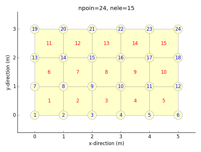
四角形要素を用いる FEM プログラム用の試験データ作成の一助とするため,矩形領域要素分割プログラムを作った.
モデル化したい矩形領域の寸法・分割数などを入力することにより,節点数・要素数・要素-節点関係・節点座標を出力する.出力確認のため,モデル図も出力している.
下の記事が,matplotlib patchesの使い方について,大変参考になる.
http://matthiaseisen.com/matplotlib/
矩形領域要素分割プログラム
出力事例
実行用スクリプトフォーマット
python py_rectmesh.py aa bb nn mm x0 y0 > out.txt
| aa | :領域のx方向長さ |
| bb | :領域のy方向長さ |
| nn | :領域のx方向分割数 |
| mm | :領域のy方向分割数 |
| x0 | :領域の左下隅のx座標 |
| y0 | :領域の左下隅のy座標 |
| out.txt | :出力ファイル名 |
実行用スクリプ事例
python py_rectmesh.py 5 3 5 3 0 0 > _test.txt
出力データ事例
出力されるのは,節点数・要素数・要素-節点関係・節点座標である.
要素-節点関係の出力列の最後に要素番号が出力されるが,これは参考データである.
また,節点座標の出力列の最後に節点番号が出力されるが,これも参考データである.
   24    15                 # number of nodes, number of elements
    1    2    8    7    1   # element-node relationship
    2    3    9    8    2   # node-1, node-2, node-3, node-4, element_number(reference)
    3    4   10    9    3
    4    5   11   10    4
    5    6   12   11    5
    7    8   14   13    6
    8    9   15   14    7
    9   10   16   15    8
   10   11   17   16    9
   11   12   18   17   10
   13   14   20   19   11
   14   15   21   20   12
   15   16   22   21   13
   16   17   23   22   14
   17   18   24   23   15
     0.000     0.000    1  # x-coordinate, y-coordinate, node_number(reference)
     1.000     0.000    2
     2.000     0.000    3
     3.000     0.000    4
     4.000     0.000    5
     5.000     0.000    6
     0.000     1.000    7
     1.000     1.000    8
     2.000     1.000    9
     3.000     1.000   10
     4.000     1.000   11
     5.000     1.000   12
     0.000     2.000   13
     1.000     2.000   14
     2.000     2.000   15
     3.000     2.000   16
     4.000     2.000   17
     5.000     2.000   18
     0.000     3.000   19
     1.000     3.000   20
     2.000     3.000   21
     3.000     3.000   22
     4.000     3.000   23
     5.000     3.000   24
出力図事例
2次元弾性骨組構造解析
プログラム概要
- このプログラムは,微小変位の仮定において2次元弾性平面骨組解析を行うものである.
- 要素として,1要素2節点,1節点3自由度(水平変位・鉛直変位・回転)を有する梁要素が用いられている.
- 荷重として,節点外力,節点強制変位,節点温度変化,要素への慣性力を扱える.
- 座標システムにおいては,右方向がx軸,上方向がy軸,反時計回りが正の回転方向としている.
- 連立一次方程式は,numpy.linalg.solve(A, b) で解いている.
- 入力データファイル,出力データファイルは,空白区切りで記載される必要があり,ファイル名はコマンドライン引数として入力する.
| 扱える境界条件 |
|---|
| 項目 | 説明 |
|---|
| 節点外力 | 載荷節点数,載荷節点番号,荷重値を指定 |
| 節点温度変化 | 全節点での温度変化量を指定. |
| 要素慣性力 | 材料特性データの中で,水平方向と鉛直方向の加速度を重力加速度に対する比で指定 |
| 節点強制変位 | 強制変位を与える節点数・節点番号および変位値を指定(ゼロ変位を含む) |
FEM解析プログラム
FEM解析実行用スクリプト
python3 py_fem_frame.py inp.txt out.txt
| inp.txt | : 入力データファイル(空白区切りデータ) |
| out.txt | : 出力データファイル(空白区切りデータ) |
入力データ書式
npoin  nele  nsec  npfix  nlod                   # Basic values for analysis
E  A  I  alpha  gamma  gkh  gkv                  # Material properties
    ..... (1 to nsec) .....                      #
node_1  node_2  isec                             # Element connectivity, material set number
    ..... (1 to nele) .....                      #
x  y  deltaT                                     # Node coordinate, temperature change of node
    ..... (1 to npoin) .....                     #
lp  fix_x  fix_y  fix_r  rdis_x  rdis_y  rdis_r  # Restricted node and restrict conditions
    ..... (1 to npfix) .....                     #
lp  fp_x  fp_y  fp_r                             # Loaded node and loading conditions
    ..... (1 to nlod) .....                      #     (omit data input if nlod=0)
| npoin, nele, nsec | : 節点数,要素数,断面特性数 |
| npfix, nlod | : 拘束節点数,載荷節点数 |
| E, A, I, alpha | : 弾性係数,断面積,断面2次モーメント,線膨張係数 |
| gamma, gkh, gkv | : 単位体積重量,水平及び鉛直方向加速度(gの比) |
| node_1, node_2, isec | : 節点1,節点2,断面特性番号 |
| x, y, deltaT | : x座標,y座標,節点温度変化量 |
| lp, fix_x, fix_y, fix_r | : 節点番号,x・y・回転方向の拘束の有無(0: 自由,1: 完全拘束) |
| rdis_x, rdis_y, rdis_r | : x・y・回転方向変位(無拘束でも0を入力) |
| lp, fp_x, fp_y, fp_r | : 節点番号,x・y・回転方向荷重 |
出力データ書式
npoin  nele  nsec npfix  nlod
    (Each value of above)
sec  E  A  I  alpha  gamma  gkh  gkv
    sec   : Material number
    E     : Elastic modulus
    A     : Section area
    I     : Moment of inertia
    alpha : Thermal expansion coefficient
    gamma : Unit weight
    gkh   : Acceleration in horizontal direction (ratio to g)
    gkv   : Acceleration in vertical direction (ratio to g)
    ..... (1 to nsec) .....
node  x  y  fx  fy  fr  deltaT  kox  koy  kor
    node   : Node number
    x      : x-coordinate
    y      : y-coordinate
    fx     : Load in x-direction
    fy     : Load in y-direction
    fr     : Moment load
    deltaT : Temperature change of node
    kox    : Index of restriction in x-direction (0: free, 1: fixed)
    koy    : Index of restriction in y-direction (0: free, 1: fixed)
    kor    : Index of restriction in rotation    (0: free, 1: fixed)
    ..... (1 to npoin) .....
node  kox  koy  kor  rdis_x  rdis_y  rdis_r
    node    : Node number
    kox     : Index of restriction in x-direction (0: free, 1: fixed)
    koy     : Index of restriction in y-direction (0: free, 1: fixed)
    kor     : Index of restriction in rotation    (0: free, 1: fixed)
    rdis_x  : Given displacement in x-direction
    rdis_y  : Given displacement in y-direction
    rdis_r  : Given displacement in rotation
    ..... (1 to npfix) .....
elem  i  j  sec
    elem : Element number
    i    : Node number of start point
    j    : Node number of end point
    sec  : Material number
    ..... (1 to nele) .....
node  dis-x  dis-y  dis-r
    node  : Node number
    dis-x : Displacement in x-direction
    dis-y : Displacement in y-direction
    dis-r : Displacement in rotation
    ..... (1 to npoin) .....
elem  N_i  S_i  M_i  N_j  S_j  M_j
    elem : Element number
    N_i  : Axial force of node-i
    S_i  : Shear force of node-i
    M_i  : Moment of node-i
    N_j  : Axial force of node-j
    S_j  : Shear force of node-j
    M_j  : Moment of node-j
    ..... (1 to nele) .....
n=(total degrees of freedom)  time=(calculation time)
| dis-x, dis-y, dis-r | : x方向変位,y方向変位,回転変位 |
| N, S, M | : 軸力,せん断力,モーメント |
| n | : 全自由度(連立方程式の元) |
| time | : 計算時間 |
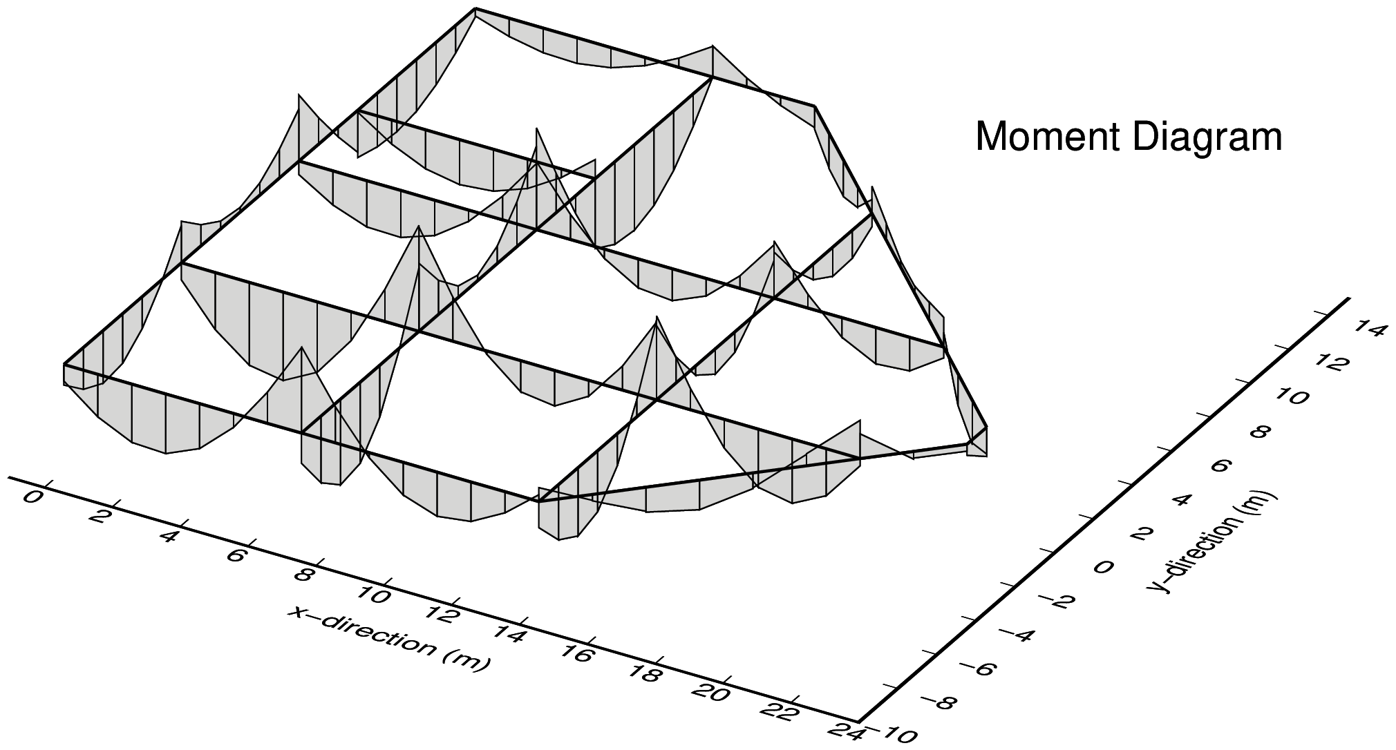
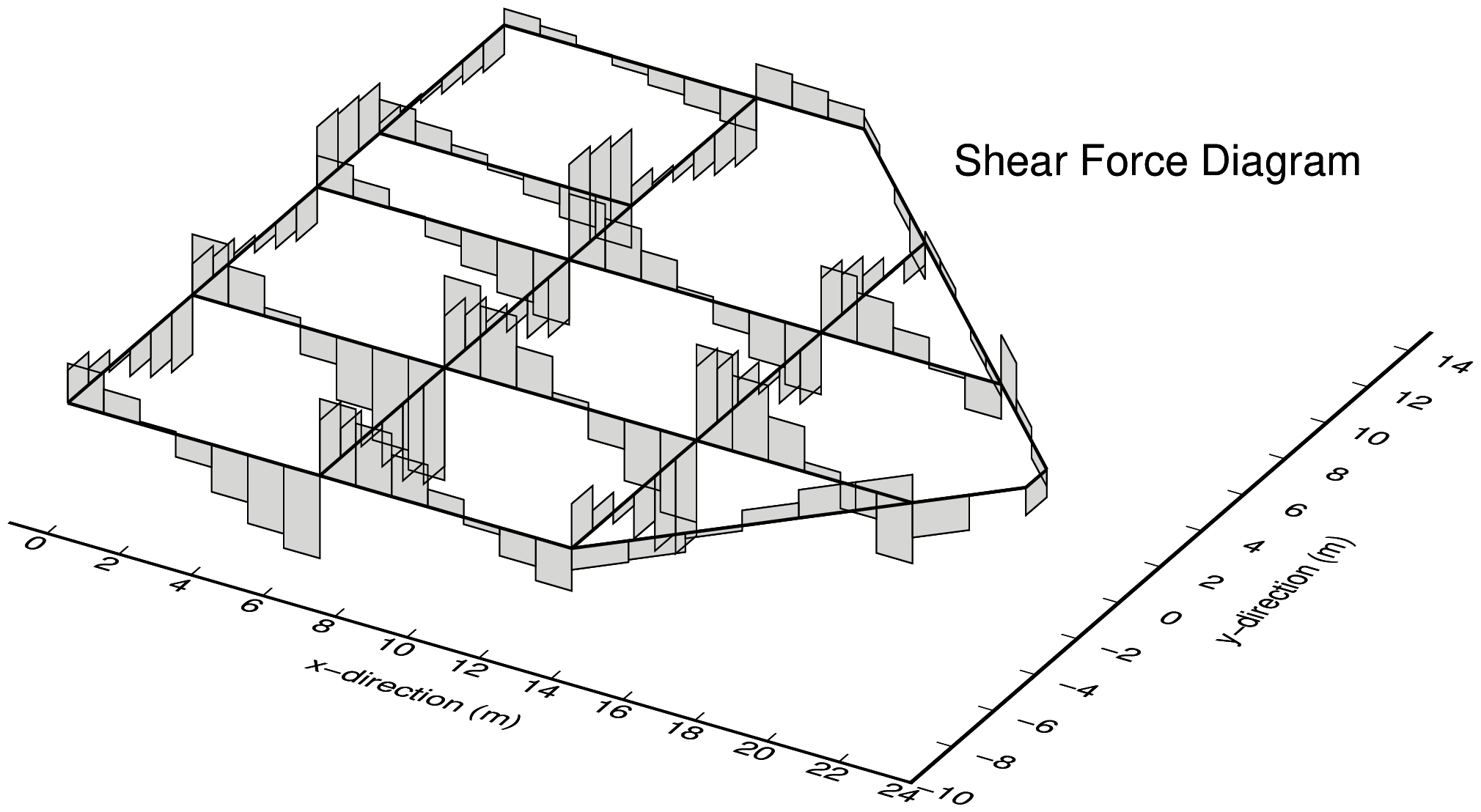
出力事例
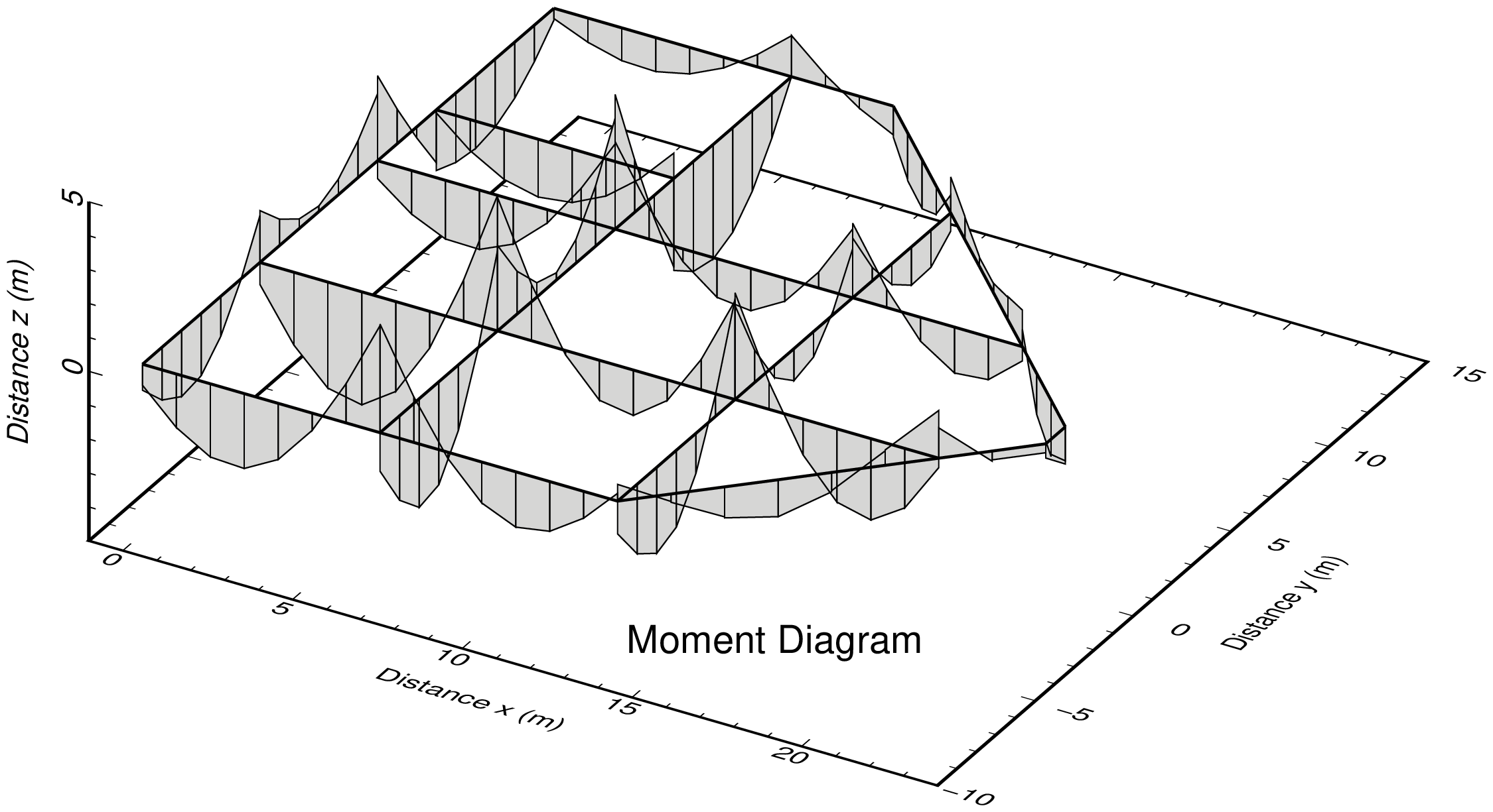
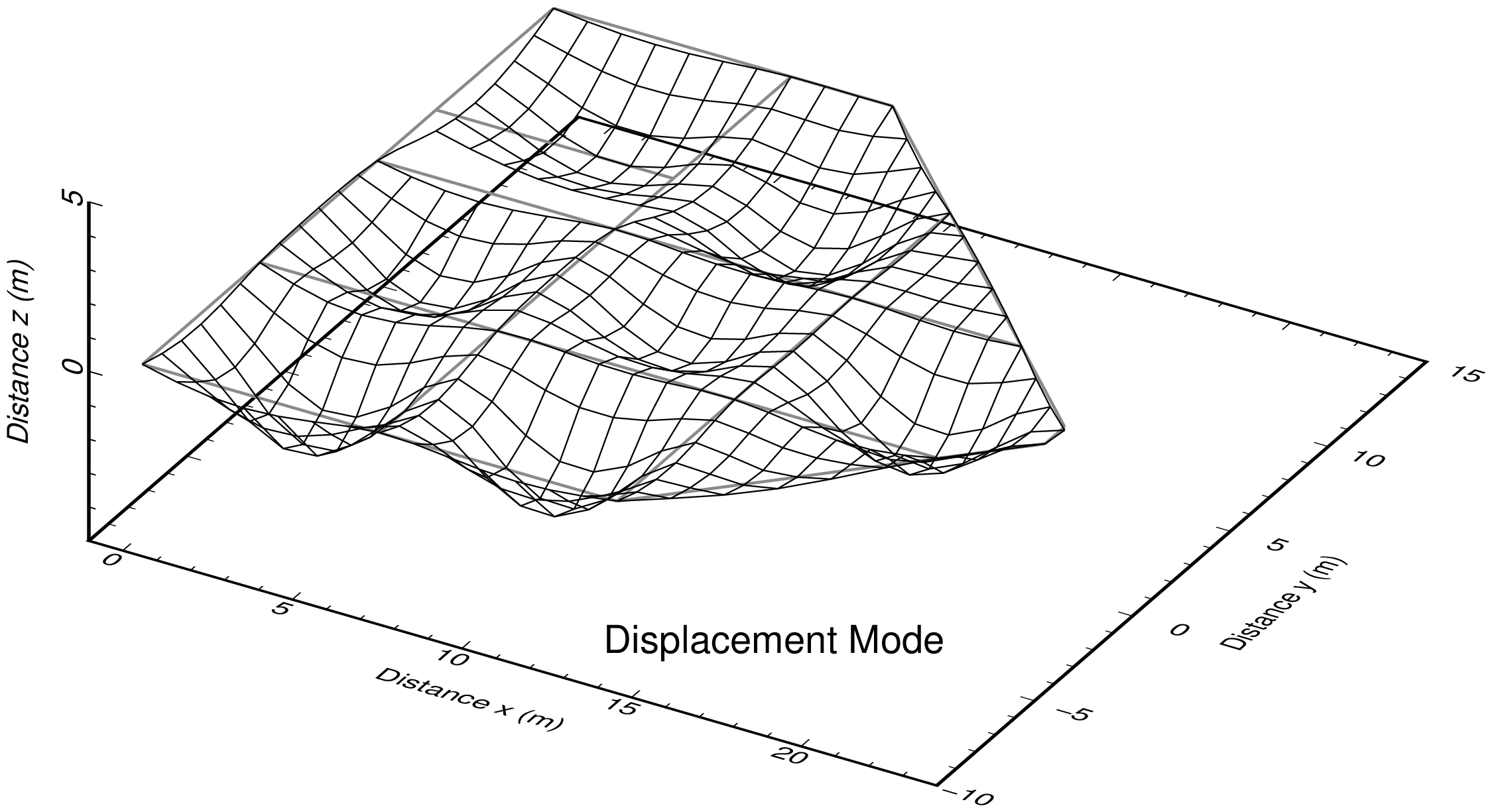
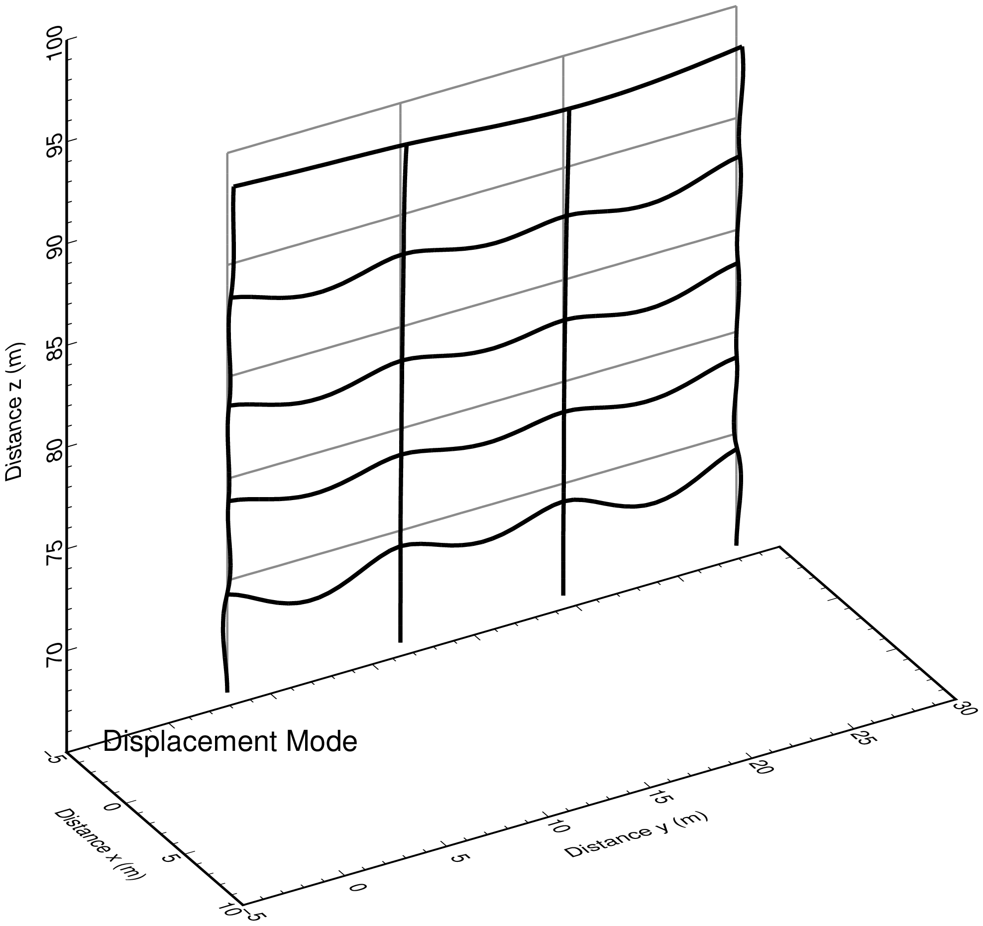
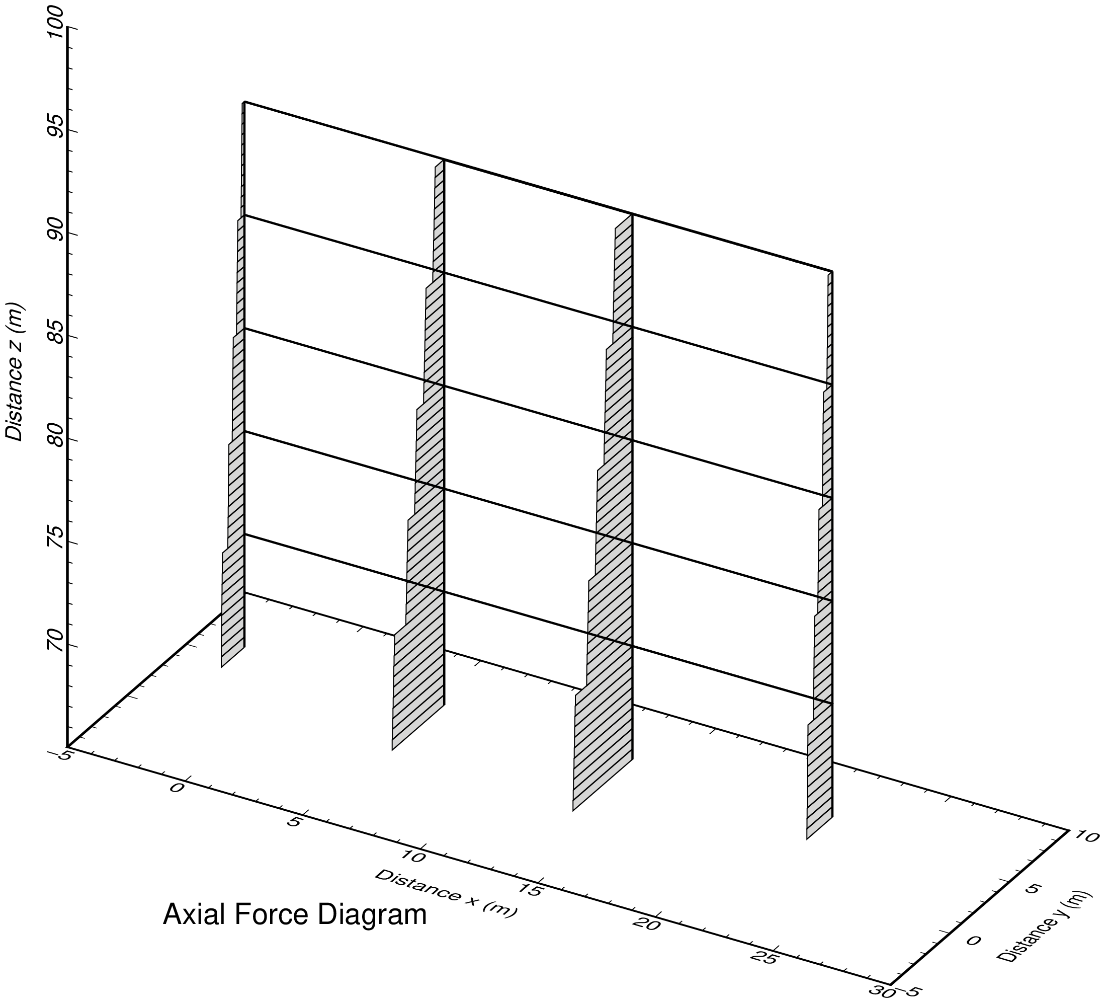
モデル概要
上載荷重,側方土圧,下部からの揚圧力を受けるコンクリート製ボックスカルバートのモデルである.3枚の壁の下端3箇所で,単純支持されている.
断面力図作成プログラム実行用スクリプト
python3 py_fem_frame.py inp_frm.tst out_frm.txt
python3 py_fig_force.py out_frm.txt
| out_frm.txt | : FEM出力データファイル(空白区切りデータ) |
この断面力図作成プログラムでは,以下の画像ファイルが自動的に作成される.
| fig_dis.png | : 変位モード図 |
| fig_axi.png | : 軸力図 |
| fig_she.png | : せん断力図 |
| fig_mom.png | : モーメント図 |
プログラムの中で,作図範囲およびスケールを指定する行は,必要に応じてモデル毎に書き換える.
axmin=np.min(x)
axmax=np.max(x)
aymin=np.min(y)
aymax=np.max(y)
midx=0.5*(axmin+axmax)
midy=0.5*(aymin+aymax)

dr=np.min([axmax-axmin,aymax-aymin])
scl_dis=0.2*dr
scl_axi=0.2*dr
scl_she=0.2*dr
scl_mom=0.3*dr
ddmax=np.max([scl_dis,scl_axi,scl_she,scl_mom])
xmin=midx-(midx-axmin+ddmax)*1.1
xmax=midx+(axmax-midx+ddmax)*1.1
ymin=midy-(midy-aymin+ddmax)*1.1
ymax=midy+(aymax-midy+ddmax)*1.6
断面力図出力事例
プログラム:py_fig_forcr.py を用い matplotlib で作成した 4 枚の png 画像を,TeX で整形して pdf 出力後,ImageMagick で png 化したものを示す.
2次元弾性トラス構造解析
プログラム概要
- このプログラムは,微小変位の仮定において2次元弾性トラス構造解析を行うものである.
- 要素として,1要素2節点,1節点2自由度(水平変位・鉛直変位)を有するトラス要素が用いられている.
- 荷重として,節点外力,節点強制変位,節点温度変化,要素への慣性力を扱える.
- 座標システムにおいては,右方向をx軸,上方向をy軸と設定している.
- 連立一次方程式は,numpy.linalg.solve(A, b) で解いている.
- 入力データファイル,出力データファイルは,空白区切りで記載される必要があり,ファイル名はコマンドライン引数として入力する.
| 扱える境界条件 |
|---|
| 項目 | 説明 |
|---|
| 節点外力 | 載荷節点数,載荷節点番号,荷重値を指定 |
| 節点温度変化 | 全節点での温度変化量を指定. |
| 要素慣性力 | 材料特性データの中で,水平方向と鉛直方向の加速度を重力加速度に対する比で指定 |
| 節点強制変位 | 強制変位を与える節点数・節点番号および変位値を指定(ゼロ変位を含む) |
FEM解析プログラム
FEM解析実行用スクリプト
python3 py_fem_truss.py inp.txt out.txt
| inp.txt | : 入力データファイル(空白区切りデータ) |
| out.txt | : 出力データファイル(空白区切りデータ) |
入力データ書式
npoin  nele  nsec  npfix  nlod    # Basic values for analysis
E  A  alpha  gamma  gkh  gkv      # Material properties
    ..... (1 to nsec) .....       #
node_1  node_2  isec              # Element connectivity, material set number
    ..... (1 to nele) .....       #
x  y  deltaT                      # Node coordinate, temperature change of node
    ..... (1 to npoin) .....      #
lp  fix_x  fix_y  rdis_x  rdis_y  # Restricted node and restrict conditions
    ..... (1 to npfix) .....      #
lp  fp_x  fp_y                    # Loaded node and loading conditions
    ..... (1 to nlod) .....       #     (omit data input if nlod=0)
| npoin, nele, nsec | : 節点数,要素数,断面特性数 |
| npfix, nlod | : 拘束節点数,載荷節点数 |
| E, A, alpha | : 弾性係数,断面積,線膨張係数 |
| gamma, gkh, gkv | : 単位体積重量,水平及び鉛直方向加速度(gの比) |
| node_1, node_2, isec | : 節点1,節点2,断面特性番号 |
| x, y, deltaT | : x座標,y座標,節点温度変化量 |
| lp, fix_x, fix_y | : 節点番号,x・y方向の拘束の有無(0: 自由,1: 完全拘束) |
| rdis_x, rdis_y | : x・y方向変位(無拘束でも0を入力) |
| lp, fp_x, fp_y | : 節点番号,x・y方向荷重 |
出力データ書式
npoin  nele  nsec npfix  nlod
    (Each value of above)
sec  E  A  alpha  gamma  gkh  gkv
    sec   : Material number
    E     : Elastic modulus
    A     : Section area
    alpha : Thermal expansion coefficient
    gamma : Unit weight
    gkh   : Acceleration in horizontal direction (ratio to g)
    gkv   : Acceleration in vertical direction (ratio to g)
    ..... (1 to nsec) .....
node  x  y  fx  fy  fr  deltaT  kox  koy  kor
    node   : Node number
    x      : x-coordinate
    y      : y-coordinate
    fx     : Load in x-direction
    fy     : Load in y-direction
    deltaT : Temperature change of node
    kox    : Index of restriction in x-direction (0: free, 1: fixed)
    koy    : Index of restriction in y-direction (0: free, 1: fixed)
    ..... (1 to npoin) .....
node  kox  koy  kor  rdis_x  rdis_y  rdis_r
    node    : Node number
    kox     : Index of restriction in x-direction (0: free, 1: fixed)
    koy     : Index of restriction in y-direction (0: free, 1: fixed)
    rdis_x  : Given displacement in x-direction
    rdis_y  : Given displacement in y-direction
    ..... (1 to npfix) .....
elem  i  j  sec
    elem : Element number
    i    : Node number of start point
    j    : Node number of end point
    sec  : Material number
    ..... (1 to nele) .....
node  dis-x  dis-y
    node  : Node number
    dis-x : Displacement in x-direction
    dis-y : Displacement in y-direction
    ..... (1 to npoin) .....
elem  N_i  S_i  N_j  S_j
    elem : Element number
    N_i  : Axial force of node-i
    S_i  : Shear force of node-i
    N_j  : Axial force of node-j
    S_j  : Shear force of node-j
    ..... (1 to nele) .....
n=(total degrees of freedom)  time=(calculation time)
| dis-x, dis-y | : x方向変位,y方向変位 |
| N, S | : 軸力,せん断力 |
| n | : 全自由度(連立方程式の元) |
| time | : 計算時間 |
格子桁構造解析
プログラム概要
- このプログラムは,微小変位の仮定において弾性格子桁構造解析を行うものである.
- 要素として,1要素2節点,1節点3自由度(ねじり回転・曲げ回転・鉛直変位)を有する梁要素が用いられている.
- 荷重として,節点外力,節点強制変位を扱える.
- 格子桁構造は,全体座標系のX-Y平面内で定義する必要がある.
- 要素座標系でのx方向は要素軸方向としている.
- 要素座標系のx軸回り回転量は,ねじりモーメントによる回転量になる.
- 要素座標系のy軸回り回転量は,曲げモーメントによる回転量になる.
- 要素座標系のz方向変位は桁のたわみになる.このたわみ量は全体座標系での値と同一である.
- 連立一次方程式は,numpy.linalg.solve(A, b) で解いている.
- 入力データファイル,出力データファイルは,空白区切りで記載される必要があり,ファイル名はコマンドライン引数として入力する.
| 扱える境界条件 |
|---|
| 項目 | 説明 |
|---|
| 節点外力 | 載荷節点数,載荷節点番号,荷重値を指定 |
| 節点強制変位 | 強制変位を与える節点数・節点番号および変位値を指定(ゼロ変位を含む) |
FEM解析プログラム
FEM解析実行用スクリプト
python3 py_fem_grid.py inp.txt out.txt
| inp.txt | : 入力データファイル(空白区切りデータ) |
| out.txt | : 出力データファイル(空白区切りデータ) |
入力データ書式
npoin  nele  nsec  npfix  nlod                   # Basic values for analysis
E  po  A  I  J                                   # Material properties
    ..... (1 to nsec) .....                      #
node_1  node_2  isec  qw                         # Element connectivity, material set number, load
    ..... (1 to nele) .....                      #
x  y                                             # Node coordinate
    ..... (1 to npoin) .....                     #
lp  fix_x  fix_y  fix_z  rdis_x  rdis_y  rdis_z  # Restricted node and restrict conditions
    ..... (1 to npfix) .....                     #
lp  fp_x  fp_y  fp_z                             # Loaded node and loading conditions
    ..... (1 to nlod) .....                      #     (omit data input if nlod=0)
| npoin, nele, nsec | : 節点数,要素数,断面特性数 |
| npfix, nlod | : 拘束節点数,載荷節点数 |
| E, po, A, I, J | : 弾性係数,ポアソン比,断面積,断面2次モーメント,ねじり定数 |
| node_1, node_2, isec, qw | : 節点1,節点2,断面特性番号,単位長さ当たり等分布鉛直荷重 |
| x, y | : x座標,y座標 |
| lp, fix_x, fix_y, fix_z | : 節点番号,ねじり・曲げ・鉛直変位の拘束の有無(0: 自由,1: 完全拘束) |
| rdis_x, rdis_y, rdis_z | : ねじり量,曲げ回転量,鉛直変位(無拘束でも0を入力) |
| lp, fp_x, fp_y, fp_z | : 節点番号,ねじりモーメント,曲げモーメント,鉛直荷重 |
解析では,せん断弾性係数が必要であるが,このプログラムの入力データは,縦弾性係数 ($E$, E) とポアソン比 ($\nu$, po) として,プログラム内で以下の関係を用いてせん断弾性係数 $G$ を算定している.
\begin{equation}
G=\cfrac{E}{2 (1+\nu)}
\end{equation}
出力データ書式
npoin  nele  nsec npfix  nlod
    (Each value of above)
sec  E  po  A  I  J
    sec   : Material number
    E     : Elastic modulus
    po    : Poisson's ratio
    A     : Section area
    I     : Moment of inertia
    J     : Tortional constant
    ..... (1 to nsec) .....
node  x  y  fx  fy  fz  kox  koy  koz
    node   : Node number
    x      : x-coordinate
    y      : y-coordinate
    fx     : Tortional moment load around x-axis
    fy     : Bending moment load
    fz     : Vertical load
    kox    : Index of restriction in tortional rotationin (0: free, 1: fixed)
    koy    : Index of restriction in bending rotation     (0: free, 1: fixed)
    koz    : Index of restriction in vertical direction   (0: free, 1: fixed)
    ..... (1 to npoin) .....
node  kox  koy  kor  rdis_x  rdis_y  rdis_r
    node    : Node number
    kox     : Index of restriction in tortional rotationin (0: free, 1: fixed)
    koy     : Index of restriction in bending rotation     (0: free, 1: fixed)
    koz     : Index of restriction in vertical direction   (0: free, 1: fixed)
    rdis_x  : Given rotation by tortional moment
    rdis_y  : Given rotation by bending moment
    rdis_z  : Given displacement in z (vertical) direction
    ..... (1 to npfix) .....
elem  i  j  sec
    elem : Element number
    i    : Node number of start point
    j    : Node number of end point
    sec  : Material number
    qw   : uniformly distributed vertical load per unit length
    ..... (1 to nele) .....
node  dis-x  dis-y  dis-r
    node  : Node number
    dis-x : Rotation by tortional moment
    dis-y : Rotation by bending moment
    dis-z : Vertical displacement
    ..... (1 to npoin) .....
elem  T_i  M_i  Q_i  T_j  M_j  Q_j
    elem : Element number
    T_i  : Tortional moment of node-i
    M_i  : Bending moment of node-i
    Q_i  : Shear force of node-i
    T_j  : Tortional moment of node-j
    M_j  : Bending moment of node-j
    Q_j  : Shear force of node-j
    ..... (1 to nele) .....
n=(total degrees of freedom)  time=(calculation time)
| dis-x, dis-y, dis-z | : ねじり回転量,曲げ回転量,鉛直変位 |
| T, M, Q | : ねじりモーメント,曲げモーメント,せん断力 |
| n | : 全自由度(連立方程式の元) |
| time | : 計算時間 |
出力事例
モデル概要
五角形の平面領域にコンクリート製の桁が配置された構造に鉛直下向き分布荷重が作用した場合の解析事例を示す.
解析実行・作図スクリプト
python3 py_fem_grid.py inp_grid.txt out_grid.txt  # FEM calculation
python3 py_grid_result.py out_grid.txt            # Data making for GMT drawings
bash a_gmt_result.txt                             # GMT script for drawing
epsをpngに変換するImageMagickコマンド(z.txt)
mogrify -trim -density 300 -bordercolor "#ffffff" -border 10x10 -format png *.eps
rm *.eps
GMTで作成した格子桁解析モデル図および荷重パターン図
使用プログラム:py_grid_model.py, a_gmt_model.txt
GMT で出力した eps 画像を ImageMagick で png 化したものを示す.
 |
 |
| 格子桁解析モデル図 | 荷重パターン図(鉛直下向き荷重) |
|---|
GMTで作成した断面力図
使用プログラム:py_grid_result.py, a_gmt_result.txt
GMT で出力した eps 画像を ImageMagick で png 化したものを示す.
3次元弾性骨組構造解析
プログラム概要
- このプログラムは,微小変位の仮定において3次元弾性平面骨組解析を行うものである.
- 要素として,1要素2節点,1節点6自由度(x-y-z方向の変位および回転)を有する梁要素が用いられている.
- 荷重として,節点外力,節点強制変位,節点温度変化,要素への慣性力を扱える.
- 全体座標系においては,鉛直上向きがZ方向,水平面をX-Y座標で構成することを想定している.
- 部材座標系においては,部材長軸方向をx軸,y軸およびz軸は断面の主軸方向を想定している.
- 連立一次方程式は,numpy.linalg.solve(A, b) で解いている.
- 入力データファイル,出力データファイルは,空白区切りで記載される必要があり,ファイル名はコマンドライン引数として入力する.
| 扱える境界条件 |
|---|
| 項目 | 説明 |
|---|
| 節点外力 | 載荷節点数,載荷節点番号,荷重値を指定 |
| 節点温度変化 | 全節点での温度変化量を指定. |
| 要素慣性力 | 材料特性データの中で,X方向・Y方向・Z方向の加速度を重力加速度に対する比で指定 |
| 節点強制変位 | 強制変位を与える節点数・節点番号および変位値を指定(ゼロ変位を含む) |
FEM解析プログラム
FEM解析実行用スクリプト
python3 py_fem_3dfrm.py inp.txt out.txt
| inp.txt | : 入力データファイル(空白区切りデータ) |
| out.txt | : 出力データファイル(空白区切りデータ) |
入力データ書式
npoin  nele  nsec  npfix  nlod                   # Basic values for analysis
E  po  A  Ix  Iy  Iz  theta  alpha  gamma  gkX  gkY  gkZ
    ..... (1 to nsec) .....                      # Material properties
node_1  node_2  isec                             # Element connectivity, material set number
    ..... (1 to nele) .....                      #
x  y  z  deltaT                                  # Node coordinate, temperature change of node
    ..... (1 to npoin) .....                     #
lp  kox  koy  koz  kmx  kmy  kmz  rdis_x  rdis_y  rdis_z  rrot_x  rrot_y  rrot_z
    ..... (1 to npfix) .....                     # Restricted node and restrict conditions
lp  fp_x  fp_y  fp_z  mp_x  mp_y  mp_z           # Loaded node and loading conditions
    ..... (1 to nlod) .....                      #     (omit data input if nlod=0)
npoin, nele, nsec       : 節点数,要素数,断面特性数
npfix, nlod             : 拘束節点数,載荷節点数
E, po, A                : 弾性係数,ポアソン比,断面積
Ix, Iy, Iz, theta       : ねじり定数,y軸回り断面二次モーメント,z軸回り断面二次モーメント,コードアングル
alpha, gamma            : 線膨張係数,材料の単位体積重量
gkX, gkY, gkZ           : X方向・Y方向・Z方向の加速度(gに対する比)
node-1, node-2, isec    : 要素を構成する節点番号,断面特性番号
x, y, z, deltaT         : 節点の(x,y,z)座標,節点温度上昇量(温度降下は負数で入力)
lp,kox,koy,koz          : 拘束節点番号,x方向・y方向・z方向拘束の有無
   kmx,kmy,kmz          : 拘束節点番号,x軸回り回転・y軸回り回転・z軸回り回転拘束の有無 (0: 無拘束, 1: 拘束)
   rdis_x,rdis_y,rdis_z : 各自由度に対する変位量を指定 (無拘束であっても0を入力)
   rrot_x,rrot_y,rrot_z : 各自由度に対する回転量を指定 (無拘束であっても0を入力)
lp, fp_x, fp_y, fp_z    : 載荷節点番号,各自由度に対する節点外力(X,Y,Z方向力)を入力
    mp_x, mp_y, mp_z    : 各自由度に対する節点外力(モーメント)を入力
出力データ書式
npoin  nele  nsec npfix  nlod
    (Each value of above)
sec  E      po     A    J    Iy    Iz    theta
sec  alpha  gamma  gkX  gkY  gkZ
    sec   : Material number
    E     : Elastic modulus
    po    : Poisson's ratio
    A     : Section area
    J     ; Torsional constant
    Iy    : Moment of inertia around y-axis
    Iz    : Moment of inertia around z-axis
    theta : Chord angle
    alpha : Thermal expansion coefficient
    gamma : Unit weight
    gkX   : Acceleration in X-direction (ratio to g)
    gkY   : Acceleration in Y-direction (ratio to g)
    gkZ   : Acceleration in Z-direction (ratio to g)
    ..... (1 to nsec) .....
node   x   y   z   fx   fy   fz   mx   my   mz  deltaT
    node   : Node number
    x      : x-coordinate
    y      : y-coordinate
    fx     : Load in X-direction
    fy     : Load in Y-direction
    fz     : Load in Z-direction
    mx     : Moment load around X-axis
    my     : Moment load around Y-axis
    mz     : Moment load around Z-axis
    deltaT : Temperature change of node
    ..... (1 to npoin) .....
node   kox   koy   koz   kmx   kmy   kmz   rdis_x   rdis_y   rdis_z   rrot_x   rrot_y   rrot_z
    node    : Node number
    kox     : Index of restriction in X-direction (0: free, 1: fixed)
    koy     : Index of restriction in Y-direction (0: free, 1: fixed)
    koz     : Index of restriction in Z-direction (0: free, 1: fixed)
    kmx     : Index of restriction in rotation around X-axis  (0: free, 1: fixed)
    kmy     : Index of restriction in rotation around Y-axis  (0: free, 1: fixed)
    kmz     : Index of restriction in rotation around Z-axis  (0: free, 1: fixed)
    rdis_x  : Given displacement in X-direction
    rdis_y  : Given displacement in Y-direction
    rdis_z  : Given displacement in Z-direction
    rrot_x  : Given displacement in rotation around X-axis
    rrot_y  : Given displacement in rotation around Y-axis
    rrot_z  : Given displacement in rotation around Z-axis
    ..... (1 to npfix) .....
elem     i     j   sec
    elem : Element number
    i    : Node number of start point
    j    : Node number of end point
    sec  : Material number
    ..... (1 to nele) .....
node   dis-x   dis-y   dis-z   rot-x   rot-y   rot-z
    node  : Node number
    dis-x : Displacement in X-direction
    dis-y : Displacement in Y-direction
    dis-z : Displacement in Z-direction
    rot-x : Rotation around X-axis
    rot-y : Rotation around Y-axis
    rot-z : Rotation around Z-axis
    ..... (1 to npoin) .....
elem nodei   N_i   Sy_i   Sz_i   Mx_i   My_i   Mz_i
elem nodej   N_j   Sy_j   Sz_j   Mx_j   My_j   Mz_j
    elem  : Element number
    nodei : First node nymber
    nodej : Second node number
    N_i   : Axial force of node-i
    Sy_i  : Shear force of node-i in y-direction
    Sz_i  : Shear force of node-i in z-direction
    Mx_i  : Moment of node-i around x-axis (torsional moment)
    My_i  : Moment of node-i around y-axis (bending moment)
    Mz_i  : Moment of node-i around z-axis (bending moment)
    N_j   : Axial force of node-j
    Sy_j  : Shear force of node-j in y-direction
    Sz_j  : Shear force of node-j in z-direction
    Mx_j  : Moment of node-j around x-axis (torsional moment)
    My_j  : Moment of node-j around y-axis (bending moment)
    Mz_j  : Moment of node-j around z-axis (bending moment)
    ..... (1 to nele) .....
n=(total degrees of freedom)  time=(calculation time)
出力事例
全体制御スクリプト
python3 py_fem_3dfrm.py inp_3dfrm_grid.txt out_3dfrm_grid.txt
python3 py_fig_3dfrm_grid.py
source a_3dfrm_grid.txt

python3 py_fem_3dfrm.py inp_3dfrm_b3_yz.txt out_3dfrm_b3_yz.txt
python3 py_fig_3dfrm_cpost1.py
source a_3dfrm_cpost1.txt

python3 py_fem_3dfrm.py inp_3dfrm_b3_xz.txt out_3dfrm_b3_xz.txt
python3 py_fig_3dfrm_cpost2.py
source a_3dfrm_cpost2.txt

rm _*
補助プログラムおよび入力データ
断面力図出力事例
入力データ:inp_3dfrm_grid.txt
入力データ:inp_3dfrm_b3_yz.txt
入力データ:inp_3dfrm_b3_xz.txt
2次元弾性応力解析
プログラム概要
- このプログラムは,微小変位の仮定において等方性材料の2次元弾性応力解析を行うものである.
- 平面歪問題および平面応力問題の双方に対応している.
- 要素として,1要素4節点,1節点2自由度(水平変位・鉛直変位)を有するアイソパラメトリック要素が用いられている.ガウス積分点は1要素4点である.
- 荷重として,節点外力,節点強制変位,節点温度変化,要素への慣性力を扱える.
- 座標システムにおいては,右方向をx軸,上方向をy軸と設定している.
- 連立一次方程式は,numpy.linalg.solve(A, b) で解いている.
- 入力データファイル,出力データファイルは,空白区切りで記載される必要があり,ファイル名はコマンドライン引数として入力する.
| 扱える境界条件 |
|---|
| 項目 | 説明 |
|---|
| 節点外力 | 載荷節点数,載荷節点番号,荷重値を指定 |
| 節点温度変化 | 全節点での温度変化量を指定. |
| 要素慣性力 | 材料特性データの中で,水平方向と鉛直方向の加速度を重力加速度に対する比で指定 |
| 節点強制変位 | 強制変位を与える節点数・節点番号および変位値を指定(ゼロ変位を含む) |
FEM解析プログラム
FEM解析実行用スクリプト
python3 py_fem_pl4.py inp.txt out.txt
| inp.txt | : 入力データファイル(空白区切りデータ) |
| out.txt | : 出力データファイル(空白区切りデータ) |
入力データ書式
npoin  nele  nsec  npfix  nlod  NSTR  # Basic values for analysis
t  E  po  alpha  gamma  gkh  gkv      # Material properties
    ..... (1 to nsec) .....           #
node1  node2  node3  node4  isec      # Element connectivity, material set number
    ..... (1 to nele) .....           #   (counter-clockwise order of node number)
x  y  deltaT                          # Coordinate, Temperature change of node
    ..... (1 to npoin) .....          #
node  kox  koy  rdisx  rdisy          # Restricted node and restrict conditions
    ..... (1 to npfix) .....          #
node  fx  fy                          # Loaded node and loading conditions
    ..... (1 to nlod) .....           #   (omit data input if nlod=0)
| npoin, nele, nsec | : 節点数,要素数,材料特性数 |
| npfix, nlod | : 拘束節点数,載荷節点数 |
| NSTR | : 応力状態(平面歪: 0,平面応力: 1) |
| t, E, po, alpha | : 板厚,弾性係数,ポアソン比,線膨張係数 |
| gamma, gkh, gkv | : 単位体積重量,水平及び鉛直方向加速度(gの比) |
| x, y, deltaT | : 節点x座標,節点y座標,節点温度変化 |
| node, kox, koy | : 拘束節点番号,x及びy方向拘束の有無(拘束: 1,自由: 0) |
| rdisx, rdisy | : x及びy方向変位(無拘束でも0を入力) |
| node, fx, fy | : 載荷重節点番号,x方向荷重,y方向荷重 |
出力データ書式
npoin  nele  nsec npfix  nlod   NSTR
    (Each value of above)
sec  t  E  po  alpha  gamma  gkh  gkv
    sec   : Material number
    t     : Element thickness
    E     : Elastic modulus
    po    : Poisson's ratio
    alpha : Thermal expansion coefficient
    gamma : Unit weight
    gkh   : Acceleration in x-direction (ratio to g)
    gkv   : Acceleration in y-direction (ratio to g)
    ..... (1 to nsec) .....
node  x  y  fx  fy  deltaT  kox  koy
    node   : Node number
    x      : x-coordinate
    y      : y-coordinate
    fx     : Load in x-direction
    fy     : Load in y-direction
    deltaT : Temperature change of node
    kox    : Index of restriction in x-direction (0: free, 1: fixed)
    koy    : Index of restriction in x-direction (0: free, 1: fixed)
    ..... (1 to npoin) .....
node  kox  koy  rdis_x  rdis_y
    node    : Node number
    kox     : Index of restriction in x-direction (0: free, 1: fixed)
    koy     : Index of restriction in y-direction (0: free, 1: fixed)
    rdis_x  : Given displacement in x-direction
    tdis_y  : Given displacement in y-direction
    ..... (1 to npfix) .....
elem  i  j  k  l  sec
    elem : Element number
    i    : Node number of start point
    j    : Node number of second point
    k    : Node number of third point
    l    : Node number of end point
    sec  : Material number
    ..... (1 to nele) .....
node  dis-x  dis-y
    node  : Node number
    dis-x : Displacement in x-direction
    dis-y : Displacement in y-direction
    ..... (1 to npoin) .....
elem  sig_x  sig_y  tau_xy  p1  p2  ang
    elem   : Element number
    sig_x  : Normal stress in x-direction
    sig_y  : Normal stress in y-direction
    tau_xy : Shear stress in x-y plane
    p1     : First principal stress
    p2     : Second principal stress
    ang    : Angle of the first principal stress
    ..... (1 to nele) .....
n=(total degrees of freedom)  time=(calculation time)
| dis-x, dis-y | : x方向変位,y方向変位 |
| sig_x, sig_y, tau_xy | : x方向直応力,y方向直応力,せん断応力 |
| p1, p2, ang | : 第一主応力,第二主応力,第一主応力の方向 |
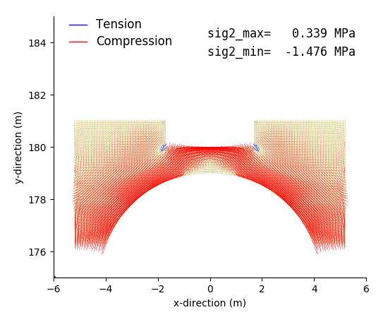
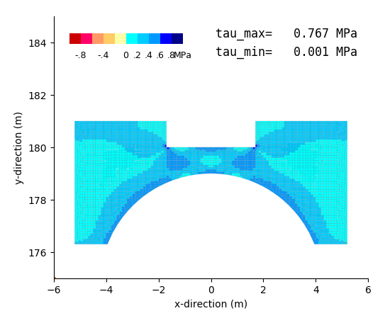
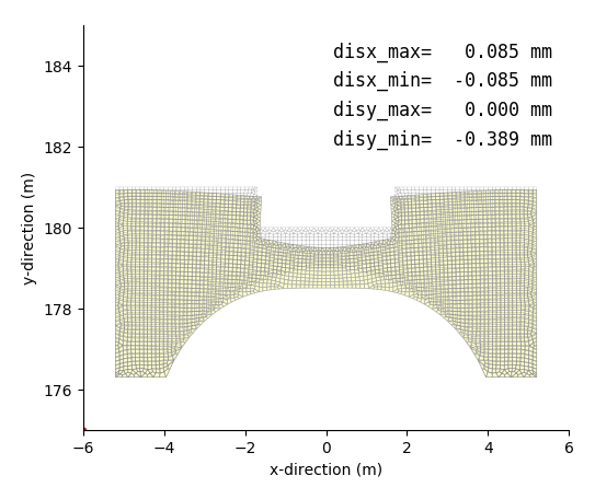
出力事例
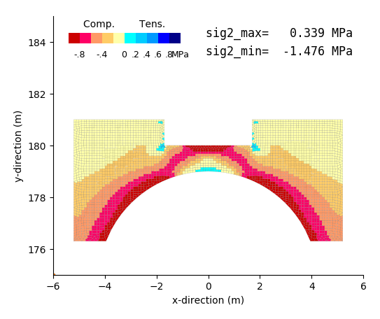
モデル概要
中央上部に切り欠きを有するコンクリートアーチの応力解析を行うもの.荷重は,上部切り欠き部の鉛直下向き分布荷重とコンクリート自重である.
FEM解析・作図実行用スクリプト
python3 py_fem_pl4.py inp_arch.txt out_arch.txt
python3 py_fig_cont_pl4.py out_arch.txt
python3 py_fig_vect_pl4.py out_arch.txt
| out_arch.txt | : FEM出力データファイル(空白区切りデータ) |
このプログラムでは,以下の画像ファイルが自動的に作成される.
py_fig_cont.py
| _fig_pl4_con1.png | : 第一主応力色分け図 |
| _fig_pl4_con2.png | : 第二主応力色分け図 |
| _fig_pl4_con3.png | : 最大せん断応力色分け図 |
py_fig_vect.py
| _fig_pl4_disp.png | : 変位モード図 |
| _fig_pl4_vec1.png | : 第一主応力ベクトル図 |
| _fig_pl4_vec2.png | : 第二主応力ベクトル図 |
これらのプログラムにおいては,作図範囲,応力値の区分と色,変位・ベクトルの大きさなどをモデルに応じて書き直す必要がある.
応力コンター・応力ベクトル・変位モード図出力事例
プログラム:py_fig_cont.py,py_fig_vect.py を用い matplotlib で作成した png 画像を示す.
 |
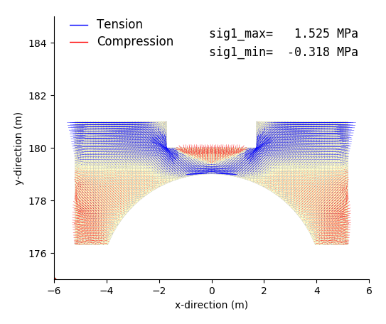 |
| First principal stress contour | First principal stress vector |
|---|
 |
 |
| Second principal stress contour | Second principal stress vector |
|---|
 |
 |
| Maximum shearing stress contour | Disolacement mode |
|---|
軸対称弾性応力解析
プログラム概要
- このプログラムは,微小変位の仮定において等方性材料の軸対称弾性応力解析を行うものである.
- 要素として,1要素4節点,1節点2自由度(回転軸方向変位・半径方向変位)を有するアイソパラメトリック要素が用いられている.ガウス積分点は1要素4点である.
- 荷重として,節点外力,節点強制変位,節点温度変化,要素への慣性力(回転軸方向のみ)を扱える.
- 座標システムにおいては,z軸を回転軸方向,r軸を半径方向に設定している.
- 連立一次方程式は,numpy.linalg.solve(A, b) で解いている.
- 入力データファイル,出力データファイルは,空白区切りで記載される必要があり,ファイル名はコマンドライン引数として入力する.
| 扱える境界条件 |
|---|
| 項目 | 説明 |
|---|
| 節点外力 | 載荷節点数,載荷節点番号,荷重値を指定 |
| 節点温度変化 | 全節点での温度変化量を指定. |
| 要素慣性力 | 材料特性データの中で,回転軸方向の加速度を重力加速度に対する比で指定 |
| 節点強制変位 | 強制変位を与える節点数・節点番号および変位値を指定(ゼロ変位を含む) |
FEM解析プログラム
FEM解析実行用スクリプト
python3 py_fem_asnt.py inp.txt out.txt
| inp.txt | : 入力データファイル(空白区切りデータ) |
| out.txt | : 出力データファイル(空白区切りデータ) |
入力データ書式
npoin  nele  nsec  npfix  nlod    # Basic values for analysis
E  po  alpha  gamma  gkz          # Material properties
    ..... (1 to nsec) .....       #
node1  node2  node3  node4  isec  # Element connectivity, material set number
    ..... (1 to nele) .....       #   (counter-clockwise order of node number)
z  r  deltaT                      # Coorinate, temperature change of node
    ..... (1 to npoin) .....      #
node  koz  kor  rdisz  rdisr      # Restricted node and restrict conditions
    ..... (1 to npfix) .....      #   (omit data input if npfix=0)
node  fz  fr                      # Loaded node and loading conditions
    ..... (1 to nlod) .....       #   (omit data input if nlod=0)
| npoin, nele, nsec | : 節点数,要素数,材料特性数 |
| npfix, nlod | : 拘束節点数,載荷節点数 |
| E, po, alpha | : 弾性係数,ポアソン比,線膨張係数 |
| gamma, gkz | : 単位体積重量,z方向加速度(gの比) |
| z, r, deltaT | : 節点z座標,節点r座標,節点温度変化 |
| node, koz, kor | : 拘束節点番号,z及びr方向拘束の有無(拘束: 1,自由: 0) |
| rdisz, rdisr | : z及びr方向変位(無拘束でも0を入力) |
| node, fz, fr | : 載荷重節点番号,z方向荷重,r方向荷重 |
荷重の考え方
例えば,半径 r=2000mm,軸方向長さ z=500mm の円筒1要素に p=1N/mm$^2$ (=1MPa) の内圧が作用する場合,要素の内壁に作用する全荷重は,以下の通りとなる.回転方向の角度は 1 ラジアンを考える.
\begin{equation}
p\times r\times 1(rad)\times z=1(N/mm^2)\times 2,000(mm)\times 1(rad)\times 500(mm)=1,000,000(N)
\end{equation}
このため,等価節点力の考え方により,(z,r)=(0,2,000) の節点に 500,000(N),(z,r)=(500,2,000) の節点に500,000(N) を半径正方向に載荷すればよいことになる.
出力データ書式
npoin  nele  nsec npfix  nlod
    (Each value of above)
sec  E  po  alpha  gamma  gkz
    sec   : Material number
    E     : Elastic modulus
    po    : Poisson's ratio
    alpha : Thermal expansion coefficient
    gamma : Unit weight
    gkz   : Acceleration in rotation axis direction (ratio to g)
    ..... (1 to nsec) .....
node  z  r  fz  fr  deltaT  koz  kor
    node   : Node number
    z      : z-coordinate (rotation axis direction)
    r      : r-coordimate (radial direction)
    fz     : Load in z-direction
    fr     : Load in r-direction
    deltaT : Temperature change of node
    koz    : Index of restriction in z-direction (0: free, 1: fixed)
    kor    : Index of restriction in r-direction (0: free, 1: fixed)
    ..... (1 to npoin) .....
node  koz  kor  rdis_z  rdis_r
    node   :
    koz    : Index of restriction in z-direction (0: free, 1: fixed)
    kor    : Index of restriction in r-direction (0: free, 1: fixed)
    rdis_z : Given displacement in z-direction
    rdis_r : Given displacement in r-direction
    ..... (1 to npfix) .....
elem  i  j  k  l  sec
    elem : Element number
    i    : Node number of start point
    j    : Node number of second point
    k    : Node number of third point
    l    : Node number of end point
    sec  : Material number
    ..... (1 to nele) .....
node  dis-z  dis-r
    node  : Node number
    dis-z : Displacement in z-direction
    dis-r : Displacement in r-direction
    ..... (1 to npoin) .....
elem  sig_z  sig_r  sig_t  tau_zr  p1  p2  ang
    elem   : Element number
    sig_z  : Normal stress in z-direction
    sig_r  : Normal stress in r-direction
    sig_t  : Normal stress in rotation (Third principal stress)
    tau_zr : Shear stress in z-r plane
    p1     : First principal stress in z-r plane
    p2     : Second principal stress in z-r plane
    ang    : Angle of the first principal stress in z-r plane
    ..... (1 to nele) .....
n=(total degrees of freedom)  time=(calculation time)
| dis-z, dis-r | : 回転軸方向変位,半径方向変位 |
| sig_z, sig_r | : 回転軸方向直応力,半径方向直応力 |
| sig_t | : 回転方向直応力(第三主応力) |
| p1, p2, ang | : z-r平面第一主応力,z-r平面第二主応力,z-r平面第一主応力の方向 |
出力事例(内水圧を受けるトーラスの応力解析)
FEM解析・作図実行用スクリプト
python3 py_fem_asnt.py inp_torus.txt out_torus.txt
python3 py_fig_data.py out_torus.txt
bash a_gmt_gra.txt
| inp_torus.txt | : FEM解析入力データファイル(空白区切りデータ) |
| out_torus.txt | : FEM解析出力データファイル(空白区切りデータ) |
理論解
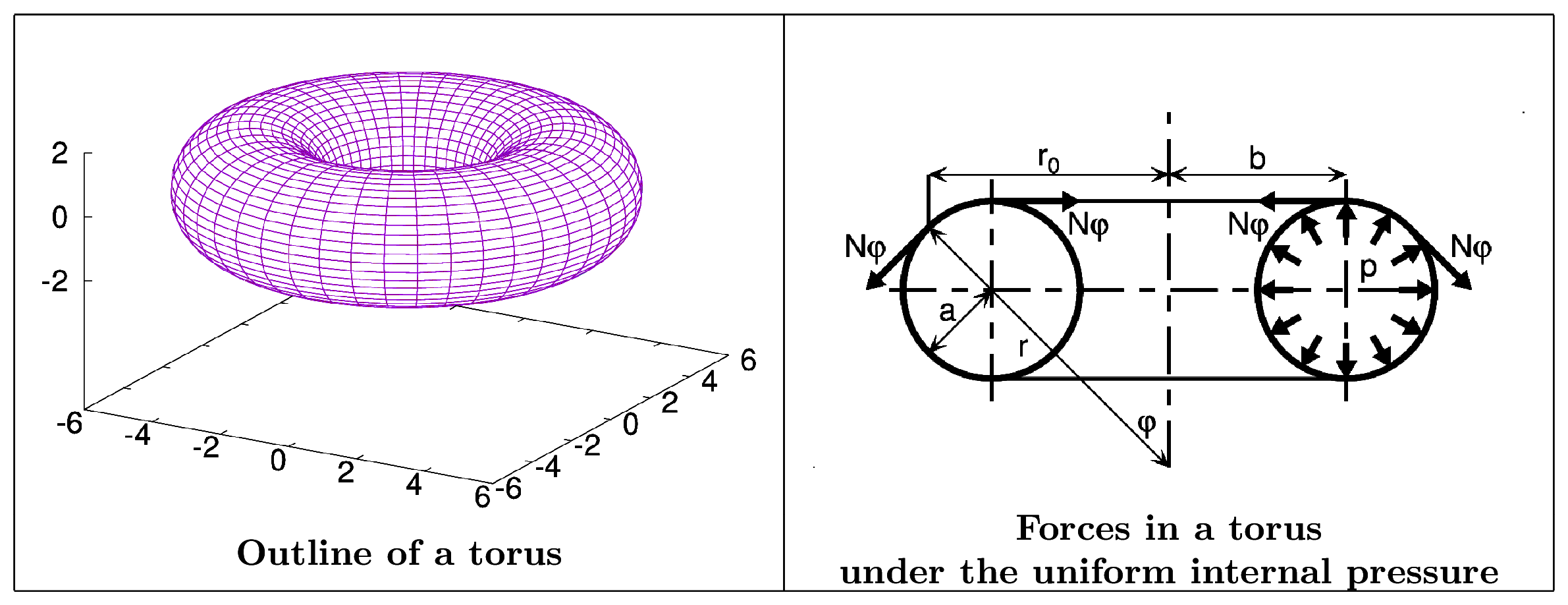
トーラス(トロイダル・シェル)とは,下図左に示すように,円環を中心軸(ここでは鉛直軸)の回りに回転させた,ドーナツ状の立体である.
上図右に示すように,均等内圧 p を受けるトーラスを考える.この場合,半径 a の円周方向軸力 $N_{\varphi}$ およびその軸方向軸力 $N_{\theta}$ は,Timoshenko (Theory of Plates and Shells) により,次式で与えられている.
\begin{equation}
N_{\varphi}=\cfrac{p a (r_0 + b)}{2 r_0} \qquad\qquad N_{\theta}=\cfrac{p a}{2}
\end{equation}
上式より,$N_{\varphi}$ は場所により変化するが,$N_{\theta}$ は,半径 a の円環上で均一な値をとることが分かる.ここで,代表点での$N_{\varphi}$を書き直してみると,
\begin{align}
&N_{\varphi}=p a \left\{1 + \cfrac{a}{2(b - a)}\right\} & (r_0 = b - a) \\
&N_{\varphi}=p a & (r_0 = b) \\
&N_{\varphi}=p a \left\{1 - \cfrac{a}{2(b + a)}\right\} & (r_0 = b + a)
\end{align}
となり,円環の内側,すなわち回転軸側 ($r_0 = b - a$) の円周方向応力が大きくなることがわかる.また,半径 a の円環の頂部と底部の円周方向応力は,通常の均等内水圧を受ける半径 a の直線円環の周方向軸力と同じ値となる.
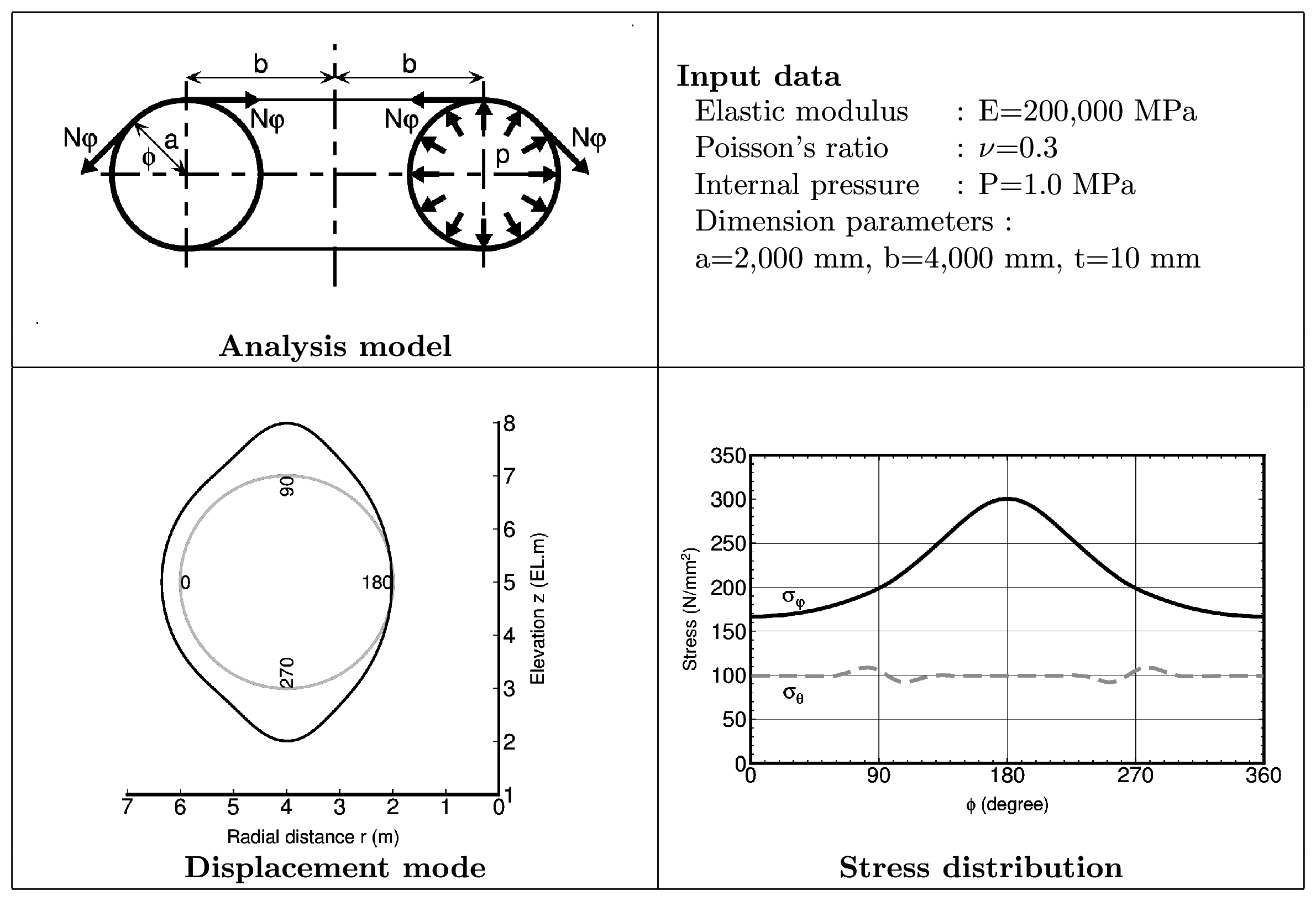
軸対称FEMによる解析
以下に示すトーラスの発生応力を,軸対称FEM解析にて予測してみた.解析条件は以下のとおり.ここに,t はトーラスを構成する材料の板厚を示す.
| E (MPa) | po | p (MPa) | a (mm) | b (mm) | t (mm) |
|---|
| 200,000 | 0.3 | 1.0 | 2,000 | 4,000 | 10 |
| 要素数:360 (半径 a の円を中心角 1 度で分割) |
軸対称FEMでは荷重は回転軸に対し 1 rad あたりの荷重を入力するようになっている.水圧についても例外ではなく,定義に忠実に荷重を作成・入力する必要があることに注意が必要である.
上図右下の応力分布図において,水平軸の角度は,変位図を参照して,トーラス外側最外点(水平左端)をゼロとして,頂部が90度,回転軸側最内点が180度,底部が270度としている.
解析結果と Timoshenko の解との比較を下表に示す.
| Location | FEM | Timoshenko |
|---|
| (φ) | σφ | σθ | σφ | σθ |
|---|
| 0 (r=b+a) | 166.59 | 99.54 | 166.66 | 100.00 |
| 90 (r=b) | 198.43 | 105.62 | 200.00 | 100.00 |
| 180 (r=b-a) | 300.54 | 99.55 | 300.00 | 100.00 |
| 応力の単位は MPa |
2次元飽和-不飽和浸透流解析
プログラム概要
- このプログラムは,等方性地盤の2次元定常飽和-不飽和浸透流解析を行うものである.非定常問題,異方性地盤は扱えない.
- このプログラムでは,鉛直断面内では飽和浸透流解析および不飽和浸透流解析が行うことができ,水平断面では飽和浸透流解析のみが行える.
- 不飽和地盤特性として Von Genuchten model を用いている.
- 要素として,1要素4節点,1節点1自由度(全水頭あるいは流量)を有するアイソパラメトリック要素が用いられている.ガウス積分点は1要素4点である.
- 地盤の奥行きは考慮できない.入力物性値の単位に応じた単位奥行きのみが考慮される.
- 境界条件として,不透水境界,全水頭指定境界,流量指定境界,浸潤面境界が扱える.
- 座標系は,x軸を右方向,z軸を上方向あるいは高標高方向に設定している.
- 連立一次方程式の解としての節点水頭は全水頭である.したがって初期水頭も全て全水頭で入力する必要がある.
- 圧力水頭は,全水頭から位置水頭を差し引くことにより計算している.
- 連立一次方程式は,numpy.linalg.solve(A, b) で解いている.
- 収束判定は,繰り返し計算過程での各節点での全水頭差が 1$\times$10$^{-6}$ 以下となったことにより行っている.収束計算における最大繰り返し数は100回に設定している.
- 入力データファイル,出力データファイルは,空白区切りで記載される必要があり,ファイル名はコマンドライン引数として入力する.
| 扱える境界条件 |
|---|
| 項目 | 説明 |
|---|
| 不透水境界 | 何も指定しなければ自動的に不透水境界になる. |
| 全水頭指定境界 | 既知全水頭を指定する節点数,節点番号,全水頭値を指定する. |
| 流量指定境界 | 既知流量を指定する節点数,節点番号,流量値を指定します.正の流量値が節点への流入,負の流量値が節点からの流出になる. |
| 浸潤点境界 | 浸潤点が出現する可能性がある範囲の節点の数,節点番号を指定する.これらの節点では,圧力水頭はゼロ以下,流量は全て流出という条件が付けられる. |
解析断面に関する補足説明
- 鉛直断面内計算か,水平断面内計算かを選択する.
- 鉛直断面計算では圧力水頭は全水頭と位置水頭の差により求める.
- 水平断面計算では圧力水頭は全水頭と同一値になる.
FEM解析プログラム
FEM解析実行用スクリプト
python3 py_fem_seep4.py inp.txt out.txt
| inp.txt | : 入力データファイル(空白区切りデータ) |
| out.txt | : 出力データファイル(空白区切りデータ) |
入力データ書式
npoin  nele  nsec  koh  koq  kou  idan  # Basic values for analysis
Ak0  alpha  em                          # Material properties
    ..... (1 to nsec) .....             #
node-1  node-2  node-3  node-4  isec    # Element connectivity
    ..... (1 to nele) .....             #   (counter-clockwise order of node number)
x  z  hvec0                             # Coordinate, initial value of total head
    ..... (1 to npoin) .....            #
nokh  Hinp                              # Node with given total head, given total head
    ..... (1 to koh) .....              #     (omit data input if koh=0)
nokq  Qinp                              # Node with given duscharge, given discharge
    ..... (1 to koq) .....              #     (omit data input if koq=0)
noku                                    # Node with saturation point
    ..... (1 to kou) .....              #     (omit data input if kou=0)
| npoin, nele, nsec | : 節点数,要素数,材料特性数 |
| koh, koq, kou | : 水頭指定節点数,流量指定節点数,浸潤境界節点数 |
| idan | : 解析断面(0: 鉛直断面,1: 水平断面) |
| Ak0 | : 要素の飽和透水係数 |
| alpa, em | : 要素の不飽和透水特性 |
| node-1, node-2, node-3, node-4, isec | : 要素を構成する節点番号,要素の材料特性番号 |
| x, z, hvec0 | : 節点のxおよびz座標,収束計算用初期水頭値 |
| nokh, Hinp | : 水頭指定節点番号および水頭値 |
| nokq, Qinp | : 流量指定節点番号および流量値 |
| noku | : 浸潤境界節点番号 |
出力データ書式
npoin  nele  nsec   koh   koq   kou  idan
    (Each value of above)
sec  Ak0  alpha  em
    Ak0   : Permeability coefficient (saturated)
    alpha : Un-saturated parameter
    em    : Un-saturated parameter
    ..... (1 to nsec) .....
node  x  z  hvec  qvec  koh  koq  kou
    node : Node number
    x    : x-coordinate
    z    : z-coordinate
    hvec : Initial total head
    qvec : Initial discharge
    koh  : Index of node with given total head (0: free, 1: fixed)
    koq  : Index of node with given discharge  (0: free, 1: fixed)
    kou  : Index of node with saturation point (0: free, 1: fixed)
    ..... (1 to npoin) .....
node Hinp
    node : Node number
    Hinp : Given total head
    ..... (1 to koh) .....
node  Qinp
    node : Node number
    Qinp : Given discharge
    ..... (1 to koq) .....
elem  i  j  k  l  sec
    elem : Element number
    i    : Node number of start point
    j    : Node number of second point
    k    : Node number of third point
    l    : Node number of end point
    sec  : Material number
    ..... (1 to nele) .....
node  hvec  pvec  qvec  koh  koq  kou
    node : Node number
    hvec : Total head
    pvec : Pressure head (Total head minus elevation of the node)
    qvec : Discharge (+: inflow, -: outflow)
    koh  : Index of node with given total head (0: free, 1: fixed)
    koq  : Index of node with given discharge  (0: free, 1: fixed)
    kou  : Index of node with saturation point (0: free, 1: fixed)
    ..... (1 to npoin) .....
elem  vx  vz  vm  kr
    elem : Element number
    vx   : Flow velocity in x-direction
    vz   : Flow velocity in z-direction
    vm   : Composed flow velocity
    kr   : Parameter of saturation (1: saturated, less than 1: unsaturated)
    ..... (1 to nele) .....
Total inflow = (total inflow discharge: positive sign)
Total outflow= (total outflow discharge: negative sign)
Max.velocity in all area     =  (maximum velocity in all area)
Max.velocity in inflow area  =  (maximum velocity in inflow area)
Max.velocity in outflow area =  (maximum velocity in outflow area)
iii=(number of itaration)
icount=(converged number of degrees of freedom)
kop=(number of pressured nodes)
n=(total degrees of freedom)  time=(calculation time)
| hvec, pvec, qvec | : 全水頭,圧力水頭,節点流量 |
| vx, vz, vm | : x方向流速,z方向流速,合成流速 |
| kr | : 飽和度パラメータ(1: 飽和,1未満: 不飽和) |
出力事例
等圧力点のプロット
考え方
自由水面は,圧力水頭が0の点を結んだものとなる.
これを可視化するための手法を示す.
基本的な考え方は以下のとおり.
- 節点座標を$(x,z)$,圧力水頭値を$y$とする.
- 3次元空間内に3点の座標値$(x_1,y_1,z_1)$,$(x_2,y_2,z_2)$,$(x_3,y_3,z_3)$を定めれば,空間中に平面Sを定義できる.
- これらの空間内の3点のうち,ある圧力水頭値$y_c$に対し,「1点の圧力が$y_c$より小+2点の圧力が$y_c$より大」,あるいは「2点の圧力が$y_c$より小+1点の圧力が$y_c$より大」の条件を満たせば,平面Sは三角形要素の面積内に$y=y_c$とする直線Lを構成する.
- ここで空間内の3点のx-z平面内の重心座標を$(x_g,z_g)$とすれば,$(x_g,z_g)$から直線Lへの最短距離とそれを与える座標$(x_x,z_z)$は,3点で構成される領域1つにつき1点,一意に定めることができる.
- この定義では,「要素重心からある直線への最短距離となる直線上の点」を求めているため,圧力水頭$y=y_c$となる点$(x_x,z_z)$は必ずしも要素内に存在するとは限らない.
計算式
3点$(x_1,y_1,z_1)$,$(x_2,y_2,z_2)$,$(x_3,y_3,z_3)$を通る空間上の平面の方程式は以下のように定義できる.
\begin{equation}
a*x+b*y+c*z+d=0
\end{equation}
\begin{align}
a=&(y_2-y_1)*(z_3-z_1)-(y_3-y_1)*(z_2-z_1) \\
b=&(z_2-z_1)*(x_3-x_1)-(z_3-z_1)*(x_2-x_1) \\
c=&(x_2-x_1)*(y_3-y_1)-(x_3-x_1)*(y_2-y_1) \\
d=&-x_1*\{(y_2-y_1)*(z_3-z_1)-(y_3-y_1)*(z_2-z_1)\} \\
&-y_1*\{(z_2-z_1)*(x_3-x_1)-(z_3-z_1)*(x_2-x_1)\} \\
&-z_1*\{(x_2-x_1)*(y_3-y_1)-(x_3-x_1)*(y_2-y_1)\}
\end{align}
また$y$がある値$y=y_c$をとる直線の方程式は以下のように定義できる.
\begin{align}
z=&-a/c*x-b/c*y_c-d/c \\
=&a'*x+b' \\
&a'=-a/c \\
&b'=-b/c*y_c-d/c
\end{align}
点$(x_g,z_g)$から直線$z=a'*x+b'$への最短距離となる直線上の点$(x_x,z_z)$は以下のとおり求められる.
\begin{equation}
\begin{cases}
&x_x=\cfrac{x_g+z_g*a'-a'*b'}{1+a'*a'} \\
&z_z=a'*x_x+b'
\end{cases}
\end{equation}
|
|
四角形要素は4節点で構成されているが,4点を通る平面は空間中に設定できない.このため,四角形要素を構成する節点を,反時計回りに4組の3点に分けて考え,ある圧力を示す点を特定することにしている.ここで要素節点番号を(1,2,3,4)とすれば,三角形を構成できる節点の組み合わせは,(1,2,3),(2,3,4),(3,4,1),(4,1,2)となる.
|
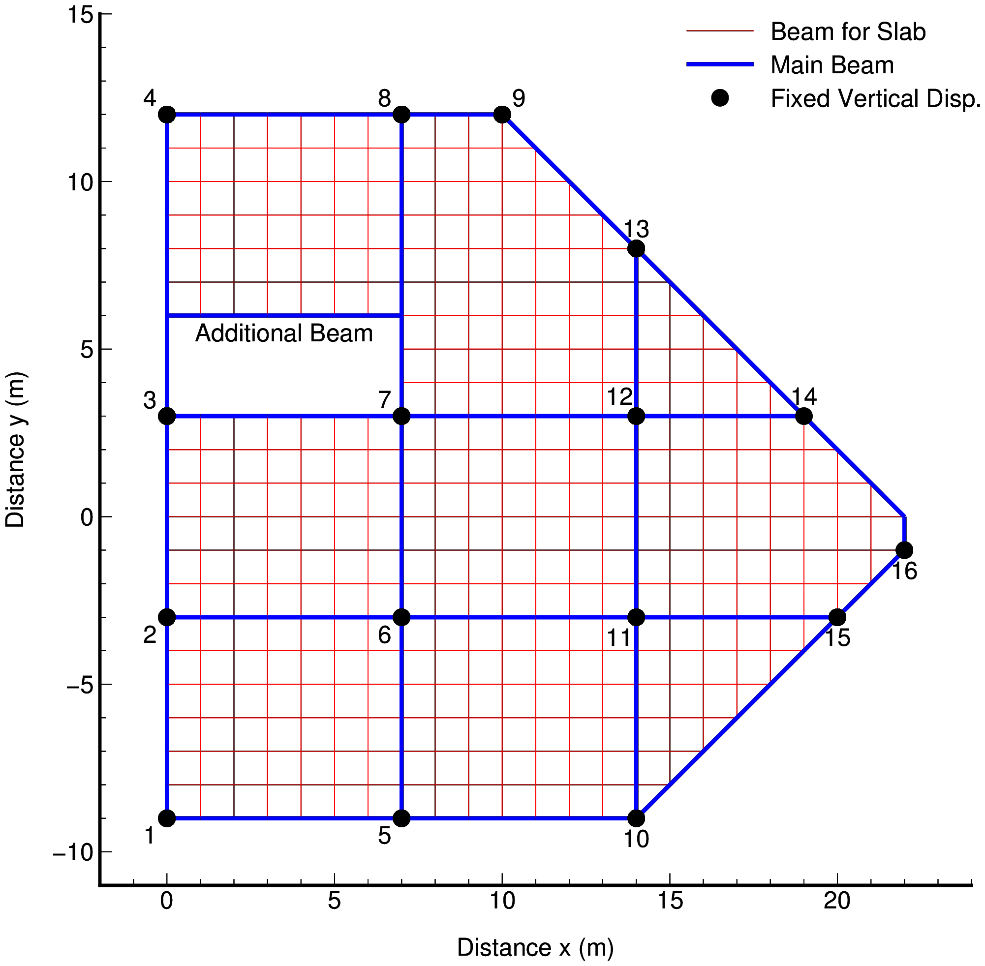
モデル概要
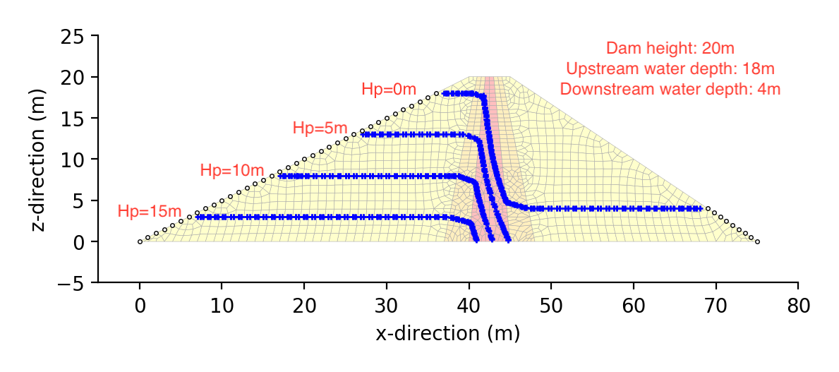
高さ20mのゾーン型ロックフィルダムの定常浸透流解析を行うもの.ダム形状,材料特性は以下に示すとおりである.
Height
(m) | Top width
(m) | Upstream
slope | Downstream
slope | Upstream
water depth (m) | Downstream
water depth (m) |
|---|
| 20.0 | 5.0 | 1:2.0 | 1:1.5 | 18.0 | 4.0 |
| Material properties |
|---|
| Zone | Permeability
k (m/s) | α
(m$^{-1}$) | m |
|---|
| Upstream shell | 1 x 10$^{-2}$ | 0.1 | 0.7 |
| Upstream filter | 1 x 10$^{-5}$ | 0.1 | 0.7 |
| Center core | 1 x 10$^{-6}$ | 0.1 | 0.7 |
| Downstream filter | 1 x 10$^{-5}$ | 0.1 | 0.7 |
| Downstream shell | 1 x 10$^{-2}$ | 0.1 | 0.7 |
FEM解析実行用スクリプト
python3 py_fem_seep4.py inp_zone4.txt out_zone4.txt
python3 py_seep4_cont.py out_zone4.txt
python3 py_seep4_vect.py out_zone4.txt
| inp_zone4.txt | : FEM解析入力データファイル(空白区切りデータ) |
| out_zone4.txt | : FEM解析出力データファイル(空白区切りデータ) |
py_seep4_cont.py は,_fig_seep4_cont.png という画像ファイルが自動的に作成される.作図範囲は一応自動設定にしてあるが,圧力コンターのピッチはプログラムを書き換えて設定する必要がある.
py_seep4_vect.py は,_fig_seep4_vect.png という画像ファイルが自動的に作成される.作図範囲は一応自動設定にしてある.
簡易圧力水頭コンター出力事例
プログラム:py_seep4_cont.py を用い,matplotlib で作成した png 画像を示す.
赤字で示した圧力水頭値(Hp=0m,5m,10m,15m)および右上黒字のダムなどの情報は,Mac のアプリケーションである Preview において,Preview $\rightarrow$ Tools $\rightarrow$ Annotate $\rightarrow$ Text で後から書き足したものである.
なお,実際のゾーン型ロックフィルダムでは,急激な水頭低下は,この解析事例のようにコアゾーン内では起こらず,コアゾーンと下流フィルターゾーンの境界で起こることが知られている.これはあくまでも解析事例ということで了解願います.
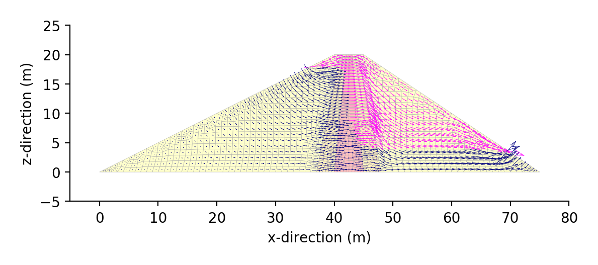
流速ベクトル図出力事例
プログラム:py_seep4_vect.py を用い,matplotlib で作成した png 画像を示す.
飽和要素の平均流速ベクトルをNavy,不飽和要素の平均流速ベクトルをMagentaで表示している.
ベクトルのプロットはquiverを用いるのが簡単なのだが,背景要素を着色するとベクトルが隠れてしまうのと,線の太さや矢印が思ったように制御できなかったので,plotを用い独自に矢印を描画している.
2次元非定常熱伝導解析
プログラム概要
- このプログラムは,等方物性を有する領域の2次元非定常熱伝導解析を行うものである.定常熱伝導問題には対応していない.
- 要素厚さは考慮できない.入力物性値の単位に応じた単位厚さのみが考慮される.
- 境界条件として,断熱境界,温度指定境界,熱伝達境界が考慮できる.
- セメント・コンクリートをモデルとした発熱体を扱うことができる.
- 要素として,1要素4節点,1節点1自由度(温度あるいは熱流束)を有するアイソパラメトリック要素が用いられている.ガウス積分点は1要素4点である.
- 座標系においては,x方向を右向き,y方向を上向きに設定している.
- 時間軸の離散化には,Crank-Nicolson method が用いられている.
- 連立一次方程式は,numpy.linalg.inv(A) で1回逆行列を求めこれを記憶して温度履歴を求めている.
- 入力データファイル,出力データファイルは,空白区切りで記載される必要があり,ファイル名はコマンドライン引数として入力する.
- 入力データファイルとして,モデル領域を定義するものと,温度指定節点温度あるいは熱伝達境界外部温度の履歴を定義するものの,2種類が必要である.
| 扱える境界条件 |
|---|
| 項目 | 説明 |
|---|
| 断熱境界 | 何も指定しなければ自動的に断熱境界となる. |
| 温度指定境界 | 既知温度履歴を指定する節点数,節点番号を指定する.また別ファイルで節点温度履歴を指定する. |
| 熱伝達境界 | 熱伝達境界を含む要素の辺の数,要素番号,辺を特定する節点番号,その辺の熱伝達率を指定する.また別ファイルで熱伝達境界の外部温度履歴を指定する. |
熱伝達境界指定に関する補足説明
熱伝達境界は,要素の辺として指定する必要がある.
このため,入力データとして,要素番号と熱伝達境界となる辺を構成する1つの節点番号を指定する.ここで,FEMでは要素を構成する節点番号は反時計回りに入力することになっているので,指定したい辺の最初の節点番号を指定することにより,その辺を特定することができる.
FEM解析プログラム
FEM解析実行用スクリプト
python3 py_fem_heat.py inp1.txt inp2.txt out.txt
| inp1.txt | : 解析モデルデータ入力ファイル(空白区切りデータ) |
| inp2.txt | : 温度指定境界温度・熱伝達境界外部温度の履歴入力ファイル(空白区切りデータ) |
| out.txt | : 出力データファイル(空白区切りデータ) |
入力データ書式
解析モデルデータ
npoin  nele  nsec  kot  koc  delta    # Basic values for analysis
Ak  Ac  Arho  Tk  Al                  # Material properties
     ..... (1 to nsec) .....          #
node-1  node-2  node-3  node-4  isec  # Element connectivity, Material set number
     ..... (1 to nele) .....          #   (counterclockwise order of node numbers)
x  y  T0                              # Coordinates of node, initial temperature of node
     ..... (1 to npoin) .....         #   (x: right-direction, y: upward direction)
nokt                                  # Node number of temperature given boundary
     ..... (1 to kot) .....           #   (Omit data input if kot=0)
nekc_0  nekc_1  alphac                # Element number, node number defined side, heat transfer rate
     ..... (1 to koc) .....           #   (Omit data input if koc=0)
n1out                                 # Number of nodes for output of temperature time history
n1node_1  ..... (1 line input) .....  # Node number for above
n2out                                 # frequency of output of temperatures of all nodes
n2step_1  ..... (1 line input) .....  # Time step number for above (Omit data input if ntout=0)
| npoin, nele, nsec | : 節点数,要素数,材料特性数 |
| kot, koc | : 温度指定境界節点数,熱伝達境界要素辺数 |
| delta | : 計算時間間隔 |
| Ak, Ac, Arho | : 熱伝導率,比熱,密度 |
| Tk, Al | : 最高断熱上昇温度,発熱速度パラメータ |
| x, y, T0 | : 節点x座標,節点y座標,節点初期温度 |
| nokt | : 温度指定境界節点番号 |
| nekc_0, nekc_1, alphac | : 熱伝達境界を有する要素番号,熱伝達境界要素辺の節点番号,熱伝達境界の熱伝達率 |
| n1out | : 全時刻歴を出力する節点数 |
| n1node | : 全時刻歴を出力する節点番号 |
| n2out | : 全節点温度を出力する時間ステップ数 |
| n2step | : 全節点温度を出力する時間ステップ番号 |
温度指定境界温度・熱伝達境界外部温度の履歴
   1   TE[1] ... TE[kot] TC[1] ... TC[koc]   # data of 1st time step
   2   TE[1] ... TE[kot] TC[1] ... TC[koc]   # data of 2nd time step
   3   TE[1] ... TE[kot] TC[1] ... TC[koc]   #
    ..... (repeating until end time) .....   #
itime  TE[1] ... TE[kot] TC[1] ... TC[koc]   #
| kot | : 温度指定境界節点数 |
| koc | : 熱伝達境界要素辺数 |
| TE[1~kot] | : 温度指定境界での温度履歴 |
| TC[1~koc] | : 熱伝達境界での外部温度履歴 |
出力データ書式
npoin  nele  nsec  kot  koc  delta  niii  n1out  n2out
    (Each value of above)
sec  Ak  Ac  Arho  Tk  Al
    sec  : Material number
    Ak   : Heat conductivity coefficient
    Ac   : Specific heat
    Arho : Unit weight
    Tk   : Maximum temperature rize
    Al   : Heat release rate
    ..... (1 to nsec) .....
node  x  y  tempe0  Tfix
    node   : Node number
    x      : x-ccordinate
    y      : y-coordinate
    tempe0 : Initial temperature
    Tfix   : Index of node with given temperature (0: free, 1: fixed)
    ..... (1 to npoin) .....
nek0  nek1  alphac
    nek0   : Element number with heat transfer boundary
    nek1   : Node number to specify heat transfer boundary side of an element
    alphac : Heat transfer rate at the specified side of an element
    ..... (1 to koc) .....
elem  i  j  k  l  sec
    elem : Element number
    i    : Node number of start point
    j    : Node number of second point
    k    : Node number of third point
    l    : Node number of end point
    sec  : Material number
    ..... (1 to nele) .....
iii  ttime  Node_(xx)  Node_(xx)  Node_(xx) .....
    iii       : Time step
    ttime     : Time
    Node-(xx) : Node number
    Time historis of each node temperature are written.
    ..... (0 to end of calculation time) .....
node  t=0.0  t=(xx)  t=(xx)0  t=(xx) .....
    node   : Node number
    t=(xx) : Specified time
    Node temperatures at specified time are written.
    ..... (1 to npoin) .....
n=(total degrees of freedom)  time=(calculation time)
出力事例
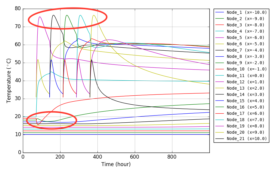
モデル概要
1辺1mの正方形領域内部に発熱体があり,周囲4辺が熱伝達境界であった場合の,領域の温度変化を予測するもの.入力物性値などの情報は以下に示すとおりである.
| Characteristics of model |
|---|
| Heat conductivity coefficient | 2.5 kcal/m h $^{\circ}$C |
| Specific heat | 0.28 kcal/kg $^{\circ}$C |
| Unit weight | 2350 kg/m$^3$ |
| Heat transfer rate | 10 kcal/m$^2$ h $^{\circ}$C |
Adiabatic temperature raise
(heating material) | $T=K\cdot(1-e^{-\alpha t})$, K=40$^{\circ}$C, α=0.2, t: hour |
| Model | 1m square area, 441 nodes, 400 elements |
| Conditions for analysis |
|---|
| Initial temperature of domain | 20 $^{\circ}$C for all nodes |
| Boundary condition | 4 sides have heat transfer boundary with outside temperature of 10 $^{\circ}$C |
| Heat generation of elements | Considered for all elements |
FEM解析実行用スクリプト
python3 py_fem_heat.py inp_div20_model.txt inp_div20_thist.txt out_div20.txt
| inp_div20_model.txt | : 解析モデルデータ入力ファイル(空白区切りデータ) |
| inp_div20_thist.txt | : 温度指定境界温度・熱伝達境界外部温度の履歴入力ファイル(空白区切りデータ) |
| out_div20.txt | : FEM解析出力データファイル(空白区切りデータ) |
温度履歴作図プログラム実行用スクリプト
python3 py_heat_2D.py out_div20.txt
このプログラムでは,_fig_tem_his.png という画像ファイルが自動的に作成される.
3次元温度分布図作成プログラム実行用スクリプト
python3 py_heat_3D.py out_div20.txt
bash _a_gmt_3D.txt
mogrify -trim -density 300 -bordercolor 'transparent' -border 10x10 -format png *.eps
rm *.eps
| _a_gmt_3D.txt | : py_heat_3D.py により作成されたGMT実行用スクリプト |
- このプログラムでは,_a_gmt_3D.txt というGMT (Generic Mapping Tools) 実行用スクリプトが自動的に作成される.
- このスクリプトを実行すると,GMTにより,_fig_gmt_xyz_0.eps, _fig_gmt_xyz_1.eps, .... というようなepsファイルが作成される.
- 上のスクリプトでは ImageMagick の mogrify コマンドにより,余白を調整しながら eps ファイルを png ファイルに書き換えている.
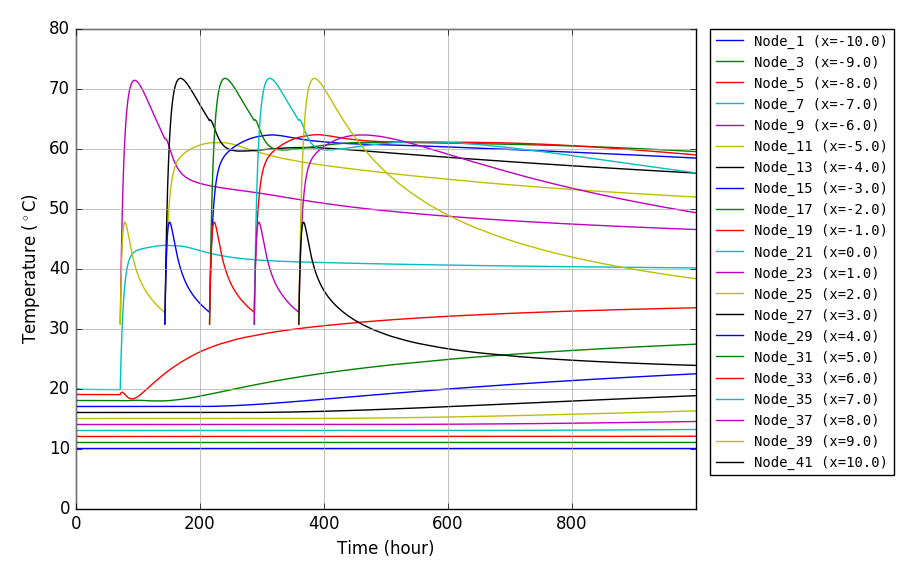
節点温度履歴図出力事例
プログラム:py_heat_2D.py を用い matplotlib で作成した png 画像を示す.
3次元温度分布図出力事例
プログラム:py_heat_3D.py を用い GMT で作成した 8 枚の eps 画像を png 化,TeX で整形して pdf 出力後,更に ImageMagick で png 化したものを示す.
2次元弾性骨組構造振動解析
時刻歴応答解析プログラム概要
- このプログラムは,微小変位の仮定において2次元弾性平面骨組構造の振動解析を行うものである.
- 要素として,1要素2節点,1節点3自由度(水平変位・鉛直変位・回転)を有する梁要素が用いられている.
- 荷重として,節点外力を扱えるが,振動加速度は1つのみしか入力できない.
節点外力として与えた数値と振動加速度の積が荷重として構造物に作用する.
- 座標システムにおいては,右方向をx軸,上方向をy軸,反時計回りを正の回転方向と設定している.
- 連立一次方程式は,numpy.linalg.inv(A) で1回逆行列を求めこれを記憶して変位の時刻歴を求めている.
- 入力データファイル,出力データファイルは,空白区切りで記載される必要があり,ファイル名はコマンドライン引数として入力する.
| 扱える境界条件 |
|---|
| 項目 | 説明 |
|---|
| 節点外力 | 載荷節点数,載荷節点番号,荷重値を指定
別ファイルで加速度を入力し,この加速度と指定した荷重値の積が構造物に載荷される |
| 節点変位拘束 | 完全拘束(ゼロ変位)のみ扱える.変位拘束する節点数・節点番号を指定 |
固有値解析プログラム概要
- このプログラムは,2次元弾性平面骨組構造の固有値解析を行い固有振動数・固有振動モードを求めるものである.
- 要素として,1要素2節点,1節点3自由度(水平変位・鉛直変位・回転)を有する梁要素が用いられている.
- 座標システムにおいては,右方向をx軸,上方向をy軸,反時計回りを正の回転方向と設定している.
- 固有方程式は,w,vr=scipy.linalg.eig(K, M) を用い一般化固有値問題として解いている.
- 入力データファイル,出力データファイルは,空白区切りで記載される必要があり,ファイル名はコマンドライン引数として入力する.
| 扱える境界条件 |
|---|
| 項目 | 説明 |
|---|
| 節点変位拘束 | 完全拘束(ゼロ変位)のみ扱える.変位拘束する節点数・節点番号を指定 |
FEM解析プログラム
時刻歴応答解析の実行用スクリプトと入出力データ書式
FEM解析実行用スクリプト
このプログラムは,指定した荷重値と加速度の積を載荷するようにしており,
入力データファイルは構造モデル用と加速度時刻歴用の2つとしている.
python3 py_fem_vfrm.py inp1.txt inp2.txr out.txt
| inp1.txt | : 構造モデル入力データファイル(空白区切りデータ) |
| inp2.txt | : 加速度時刻歴入力データファイル(空白区切りデータ) |
| out.txt | : 出力データファイル(空白区切りデータ) |
入力データ書式
npoin  nele  nsec  npfix  nlod                   # Basic values for analysis
E  A  I  gamma  zeta_m  zeta_k                   # Material properties
    ..... (1 to nsec) .....                      #
node_1  node_2  isec                             # Element connectivity, material set number
    ..... (1 to nele) .....                      #
x  y                                             # Node coordinate
    ..... (1 to npoin) .....                     #
lp  fix_x  fix_y  fix_r                          # Restricted node and restrict conditions
    ..... (1 to npfix) .....                     #
lp  fp_x  fp_y  fp_r                             # Loaded node and loading conditions
    ..... (1 to nlod) .....                      #     (omit data input if nlod=0)
| npoin, nele, nsec | : 節点数,要素数,断面特性数 |
| npfix, nlod | : 拘束節点数,載荷節点数 |
| E, A, I, gamma | : 弾性係数,断面積,断面2次モーメント,単位体積重量 |
| zeta_m, zeta_k | : Rayleigh減衰を表す係数 |
| node_1, node_2, isec | : 節点1,節点2,断面特性番号 |
| x, y | : x座標,y座標 |
| lp, fix_x, fix_y, fix_r | : 節点番号,x・y・回転方向の拘束の有無(0: 自由,1: 完全拘束) |
| lp, fp_x, fp_y, fp_r | : 節点番号,x・y・回転方向荷重 |
出力データ書式
npoin  nele  nsec  npfix  nlod  ndoutx  ndouty  nfout  delta  nnn
    (Each value of above)
sec  E  A  I  gamma  zeta_m  zeta_k
    sec    : Material number
    E      : Elastic modulus
    A      : Section area
    I      : Moment of inertia
    gamma  : Unit weight
    zeta_m : Coefficient of Rayleigh damping for mass matrix
    zeta_k : Coefficient of Rayleigh damping for stiffness matrix
    ..... (1 to nsec) .....
node  x  y  fx  fy  fr  kox  koy  kor
    node   : Node number
    x      : x-coordinate
    y      : y-coordinate
    fx     : Load in x-direction
    fy     : Load in y-direction
    fr     : Moment load
    kox    : Index of restriction in x-direction (0: free, 1: fixed)
    koy    : Index of restriction in y-direction (0: free, 1: fixed)
    kor    : Index of restriction in rotation    (0: free, 1: fixed)
    ..... (1 to npoin) .....
elem  i  j  sec
    elem : Element number
    i    : Node number of start point
    j    : Node number of end point
    sec  : Material number
    ..... (1 to nele) .....
step  time  acc_inp  dis_x(ii) vel_x(ii) acc_x(ii)  Ni(ne)node  Si(ne)  Mi(ne)
    step      : Time step
    time      : Time
    acc_inp   : Input acceleration
    dis_x(ii) : Displacement in x-direction at node-ii
    vel_x(ii) : Velocity in x-direction at node-ii
    acc_x(ii) : Acceleration in x-direction at node-ii
    Ni(ne)    : Axial force at node-i in element-ne
    Si(ne)    : Shear force at node-i in element-ne
    Mi(ne)    : Moment at node-i in element-ne
    ..... (to end of time step) .....
n=(total degrees of freedom)  time=(calculation time)
| time, acc_inp | : 経過時間,入力地盤加速度 |
| dis, vel, acc | : 変位,速度,加速度 |
| N, S, M | : 軸力,せん断力,モーメント |
| n | : 全自由度(連立方程式の元) |
| time | : 計算時間 |
固有値解析の実行用スクリプトと入出力データ書式
FEM解析実行用スクリプト
python3 py_fem_efrm.py inp.txt out.txt
| inp.txt | : 構造モデル入力データファイル(空白区切りデータ) |
| out.txt | : 出力データファイル(空白区切りデータ) |
入力データ書式
npoin  nele  nsec  npfix         # Basic values for analysis
E  A  I  gamma                   # Material properties
    ..... (1 to nsec) .....      #
node_1  node_2  isec             # Element connectivity, material set number
    ..... (1 to nele) .....      #
x  y                             # Node coordinate
    ..... (1 to npoin) .....     #
lp  fix_x  fix_y  fix_r          # Restricted node and restrict conditions
    ..... (1 to npfix) .....     #
| npoin, nele, nsec | : 節点数,要素数,断面特性数 |
| npfix | : 拘束節点数 |
| E, A, I, gamma | : 弾性係数,断面積,断面2次モーメント,単位体積重量 |
| node_1, node_2, isec | : 節点1,節点2,断面特性番号 |
| x, y | : x座標,y座標 |
| lp, fix_x, fix_y, fix_r | : 節点番号,x・y・回転方向の拘束の有無(0: 自由,1: 完全拘束) |
出力データ書式
npoin  nele  nsec  npfix
    (Each value of above)
sec  E  A  I  gamma
    sec    : Material number
    E      : Elastic modulus
    A      : Section area
    I      : Moment of inertia
    gamma  : Unit weight
    ..... (1 to nsec) .....
node  x  y  kox  koy  kor
    node   : Node number
    x      : x-coordinate
    y      : y-coordinate
    kox    : Index of restriction in x-direction (0: free, 1: fixed)
    koy    : Index of restriction in y-direction (0: free, 1: fixed)
    kor    : Index of restriction in rotation    (0: free, 1: fixed)
    ..... (1 to npoin) .....
elem  i  j  sec
    elem : Element number
    i    : Node number of start point
    j    : Node number of end point
    sec  : Material number
    ..... (1 to nele) .....
Order         1       2       3  ......
fn(Hz)      w[1]   w[2]    w[3]  ......
v[  1]   v[1,1]  v[1,2]  v[1,3]  ......
v[  2]   v[1,1]  v[1,2]  v[1,3]  ......
......   ......  ......  ......  ......
v[  n]   v[1,1]  v[1,2]  v[1,3]  ......
    Order  Ranking
    w[i]      : Natural frequency (eigen value)
    v[j,i]    : Element of eigen vector
n=(total degrees of freedom)  time=(calculation time)
(注意事項)
固有値解析プログラムにおいては,拘束節点の処理は時刻歴解析と同様にマトリックスを縮小せず,全自由度の次元を保っている.このため,拘束された自由度に相当する固有値は,昇順に並び替えると下に示すように小さい側に集まっており,かつ同じ値を示す.
この固有値に相当する固有ベクトルは,拘束された自由度の箇所に1が,それ以外は0が入った特殊なベクトルとなっている.この性質を利用し,出力時は,拘束された自由度に相当する固有値・固有ベクトルは出力しないようにしている.
[  1.59154943e-01   1.59154943e-01   1.59154943e-01   1.59154943e-01
   1.59154943e-01   1.59154943e-01   1.59154943e-01   1.59154943e-01
   1.59154943e-01   1.59154943e-01   1.59154943e-01   1.59154943e-01
   1.59154943e-01   2.35776685e+00   1.47763490e+01   4.13833696e+01
   8.11515057e+01   1.34359374e+02   2.01285622e+02   2.82413495e+02
   3.78356230e+02   4.89209902e+02   6.08158484e+02   8.09431960e+02
   9.77895783e+02   1.18543706e+03   1.43074344e+03   1.71924912e+03
   2.05623517e+03   2.44043231e+03   2.84908857e+03   3.20838993e+03
   4.01526229e+03]
出力事例(ガウス波)
FEM以外の補助プログラム
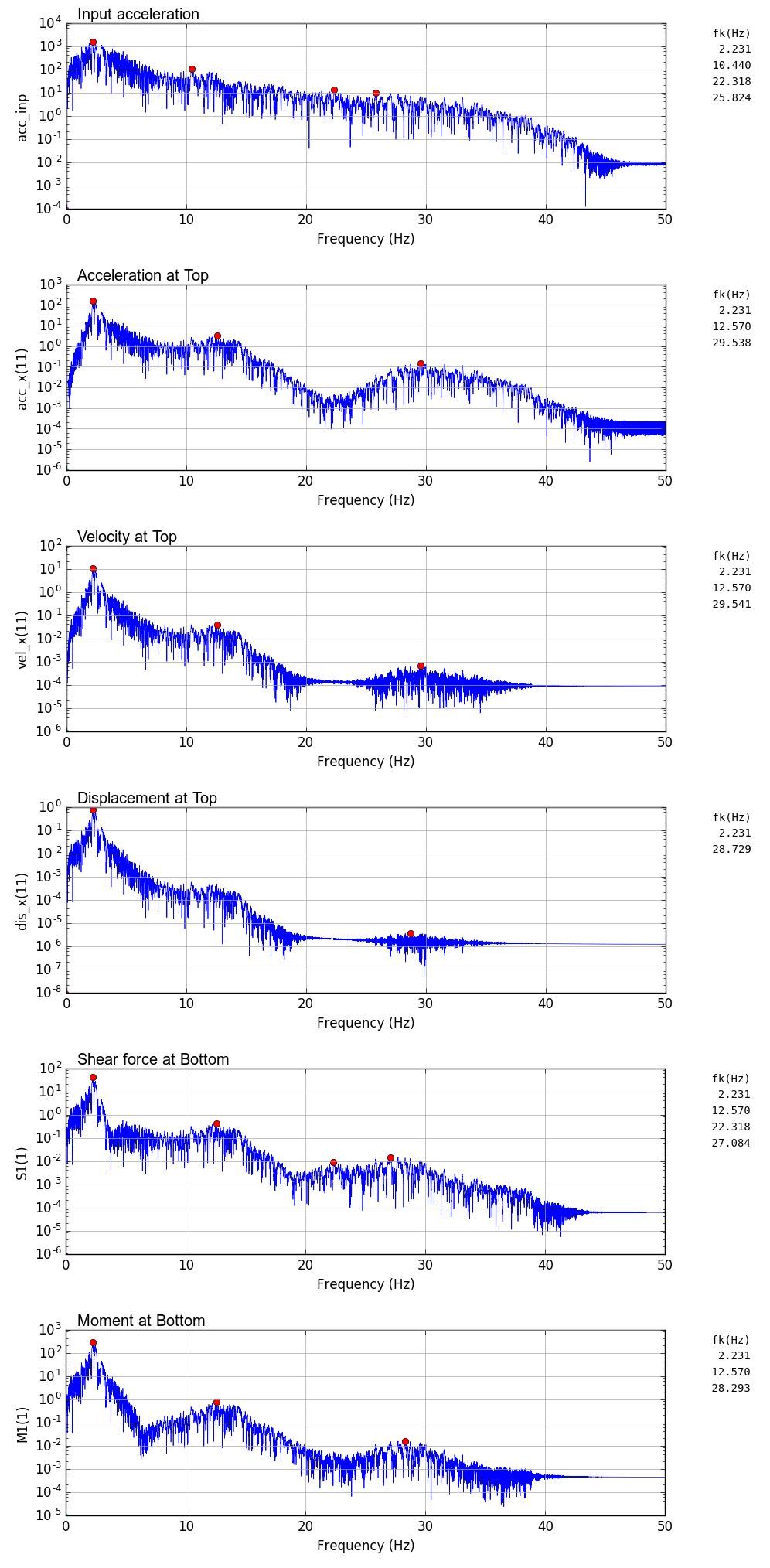
時刻歴図・フーリエスペクトル図作成プログラム(py_fig_vfrm.py)
- matplotlib で節点加速度・速度・変位・断面力の時刻歴図およびフーリエスペクトル図を作成する.
- 高速フーリエ変換には,numpy の fft を用いている.
- 卓越振動数(固有振動数)検索には,scipy の argrelmax(sp0,order=100) を用いている.
ここで sp0 は fft で求めたフーリエスペクトル,order=100 は検索する極大値を探す幅を調整するパラメータである.
入力用ガウス波作成プログラム(py_gauss.py)
- コマンドラインで入力した時間刻みでのガウス波を作成する.
- ガウス波は,0.5 秒に中心を持ち標準偏差 0.001,最大加速度 100gal に設定している.
テキスト追加プログラム(py_im.py)
- matplotlib で作成し ImageMagick で結合したpng画像に,後からテキストを加えるために作成したもの.
- Python のプログラムであるが,処理は os.system(cmd) により,ImageMagick のコマンドを呼び出して行っている.
片持梁曲げ固有振動数計算プログラム(py_fn_canti.py)
- 片持梁曲げ固有振動数計算では $\cos x \cdot \cosh x + 1 =0$ という形の非線形方程式を解く必要があるので,scipy の optimize.brentq を用いている.
- 上記非線形方程式は,cos関数の性質から,0〜π π〜2π ... と周期的に解を持つので,この性質を利用して,brentq に初期値を与えている.
固有振動モード作図プログラム(py_fig_efrm_mode.py)
- 振動固有値解析結果から matplotlib を用い,固有振動モード図を作成するプログラムである.
モデル概要
基部を完全固定された鉛直片持梁モデルが基部で水平地盤加速度を受けるモデルである.
加速度を受けるのは基部であるが,基部は固定されているため,全節点に水平方向の地盤加速度値をかけるよう入力する.
構造モデル入力データ事例
基部を完全固定された鉛直片持梁モデルである.
構造寸法や材料特性の単位は,m系である.
荷重の値は,加速度に乗じる係数として入力する.
構造物の寸法単位はmとしている($g=9.8m/s^2$ で固定)ので,入力地盤加速度の単位が gal (cm/s^2) なら荷重値は 0.01 となる.
11  10  1  1  11                    # Basic data
2000000  0.25  0.005208  2.3  0  0  # E  A  I  gamma  zeta_m  zeta_k
 1   2  1                           # Element-node relationship, material No.
 2   3  1                           #
 3   4  1                           #
 4   5  1                           #
 5   6  1                           #
 6   7  1                           #
 7   8  1                           #
 8   9  1                           #
 9  10  1                           #
10  11  1                           #
0  0                                # x, y-coordimates
0  1                                #
0  2                                #
0  3                                #
0  4                                #
0  5                                #
0  6                                #
0  7                                #
0  8                                #
0  9                                #
0  10                               #
1  1  1  1                          # Node No, restrict conditions
 1  0.01  0  0                      # Node number and Loading condition
 2  0.01  0  0                      #
 3  0.01  0  0                      # In this case, all nodes are loaded
 4  0.01  0  0                      # in x-direction.
 5  0.01  0  0                      # The values 0.01 means the coefficient
 6  0.01  0  0                      # for the input acceleration.
 7  0.01  0  0                      # Since the unit of input acceleration
 8  0.01  0  0                      # is 'gal' (cm/s^2) usually,
 9  0.01  0  0                      # the coefficient should be 0.01
10  0.01  0  0                      # because the unit of structural dimensions
11  0.01  0  0                      # are 'm'
1                                   # Number of nodes for x-dir. output (ndoutx)
11                                  # Node for dis-vel-acc output
0                                   # Number of nodes for y-dir. output (ndouty)
1                                   # Number of nodes for section force output (nfout)
1  1                                # Element and node (node should be 1 or 2)
地盤加速度入力データ事例
プログラム py_gauss.py で作成したもの.最大加速度 100 gal で t=0.5 秒に中心が来るガウス波である.
0.01                   # time increment (sec)
0.0                    # start of acceleration time history
0.0
0.0

......

3.69388306849e-194
1.38389652674e-85
1.92874984796e-20
100.0                 # 100 gal at t=0.5sec
1.92874984796e-20
1.38389652674e-85
3.69388306848e-194

......

0.0
0.0
0.0
実行用スクリプト
- py_gauss.py で時間間隔を指定して入力地盤加速度データを作成する.
- py_fem_vfrm.py でFEMによる時刻歴応答計算を行う.
- py_fig_vfrm.py で,時刻歴図およびフーリエスペクトル図を作成する.
- 作成した図面は,ケース毎に ImageMagick の convert -append により結合し1枚の画像にしている.
#dt=0.001
python py_gauss.py 0.001 > inp_gauss.txt
python py_fem_vfrm.py inp_vfrm.txt inp_gauss.txt out_vfrm.txt
python py_fig_vfrm.py out_vfrm.txt

convert -append _fig_fft_acc_inp.png _fig_fft_acc_x\(11\).png _1.png
convert -append _1.png _fig_fft_vel_x\(11\).png _2.png
convert -append _2.png _fig_fft_dis_x\(11\).png _3.png
convert -append _3.png _fig_fft_S1\(1\).png _4.png
convert -append _4.png _fig_fft_M1\(1\).png fig_fft_001.png

convert -append _fig_his_acc_inp.png _fig_his_acc_x\(11\).png _1.png
convert -append _1.png _fig_his_vel_x\(11\).png _2.png
convert -append _2.png _fig_his_dis_x\(11\).png _3.png
convert -append _3.png _fig_his_S1\(1\).png _4.png
convert -append _4.png _fig_his_M1\(1\).png fig_his_001.png

#dt=0.005
python py_gauss.py 0.005 > inp_gauss.txt
python py_fem_vfrm.py inp_vfrm.txt inp_gauss.txt out_vfrm.txt
python py_fig_vfrm.py out_vfrm.txt

convert -append _fig_fft_acc_inp.png _fig_fft_acc_x\(11\).png _1.png
convert -append _1.png _fig_fft_vel_x\(11\).png _2.png
convert -append _2.png _fig_fft_dis_x\(11\).png _3.png
convert -append _3.png _fig_fft_S1\(1\).png _4.png
convert -append _4.png _fig_fft_M1\(1\).png fig_fft_005.png

convert -append _fig_his_acc_inp.png _fig_his_acc_x\(11\).png _1.png
convert -append _1.png _fig_his_vel_x\(11\).png _2.png
convert -append _2.png _fig_his_dis_x\(11\).png _3.png
convert -append _3.png _fig_his_S1\(1\).png _4.png
convert -append _4.png _fig_his_M1\(1\).png fig_his_005.png

#dt=0.01
python py_gauss.py 0.01 > inp_gauss.txt
python py_fem_vfrm.py inp_vfrm.txt inp_gauss.txt out_vfrm.txt
python py_fig_vfrm.py out_vfrm.txt

convert -append _fig_fft_acc_inp.png _fig_fft_acc_x\(11\).png _1.png
convert -append _1.png _fig_fft_vel_x\(11\).png _2.png
convert -append _2.png _fig_fft_dis_x\(11\).png _3.png
convert -append _3.png _fig_fft_S1\(1\).png _4.png
convert -append _4.png _fig_fft_M1\(1\).png fig_fft_010.png

convert -append _fig_his_acc_inp.png _fig_his_acc_x\(11\).png _1.png
convert -append _1.png _fig_his_vel_x\(11\).png _2.png
convert -append _2.png _fig_his_dis_x\(11\).png _3.png
convert -append _3.png _fig_his_S1\(1\).png _4.png
convert -append _4.png _fig_his_M1\(1\).png fig_his_010.png

rm _*
固有値解析入力データ
鉛直片持梁の曲げ振動固有値解析用データを以下に示す.
固有値解析においては,荷重の入力がないため,y(水平)方向を拘束しないと,縦振動のモードを含んで固有値を求めてしまう.ここでは,曲げ振動の固有値のみがほしいので,全節点において,水平方向変位を拘束(ゼロセット)している.
11  10  1  11                 # npoin nele nsec npfix
2000000  0.25  0.005208  2.3  # Material properties
 1   2  1                     # Element-node relationship
 2   3  1                     #    and material number
 3   4  1                     #
 4   5  1                     #
 5   6  1                     #
 6   7  1                     #
 7   8  1                     #
 8   9  1                     #
 9  10  1                     #
10  11  1                     #
0  0                          # x, y-coordinate
0  1                          #
0  2                          #
0  3                          #
0  4                          #
0  5                          #
0  6                          #
0  7                          #
0  8                          #
0  9                          #
0  10                         #
1  1  1  1                    # Restrict conditions
2  0  1  0                    # Node-1: all are restricted
3  0  1  0                    #     because of fixed edge.
4  0  1  0                    # Node-2 to 11:
5  0  1  0                    #    y(horizontal)-direction are restricted
6  0  1  0                    #    becasu of to eliminate the effect of
7  0  1  0                    #    axial displacement.
8  0  1  0                    #
9  0  1  0                    #
10 0  1  0                    #
11 0  1  0                    #
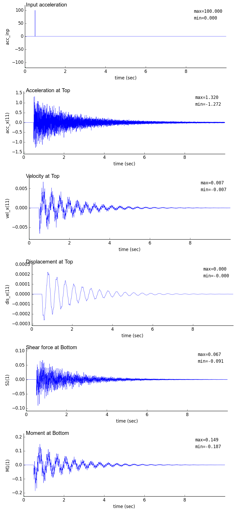
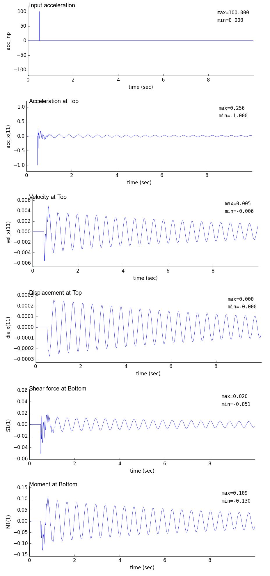
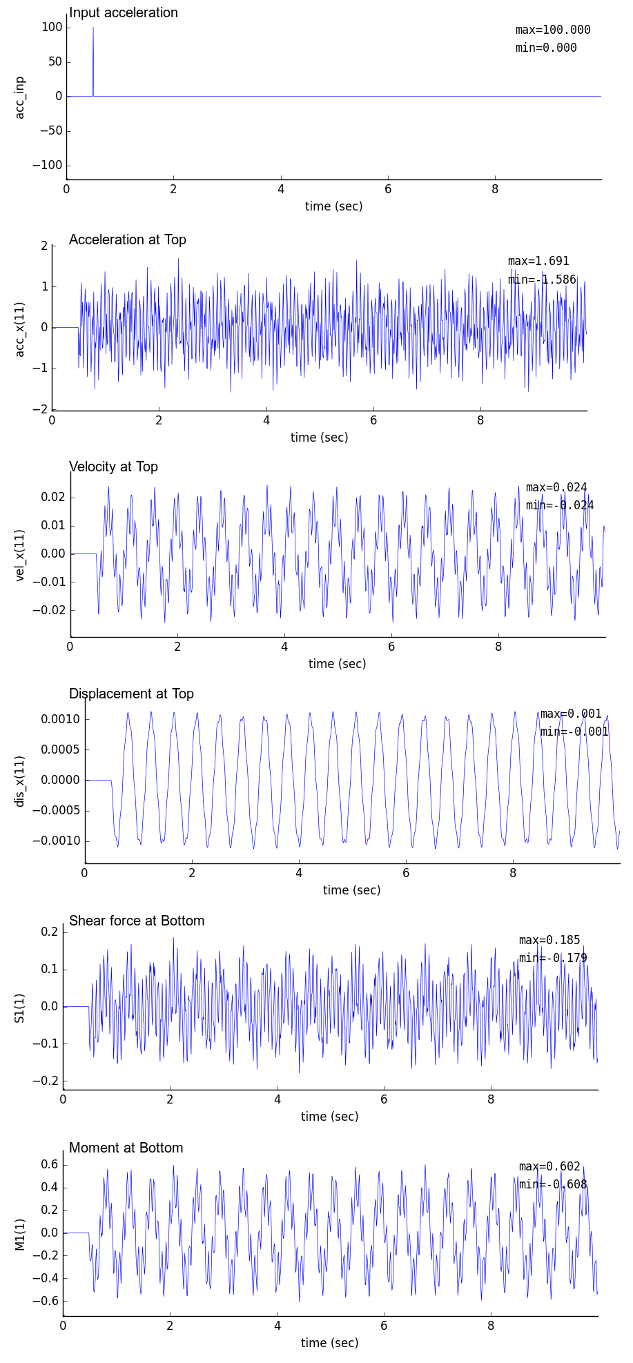
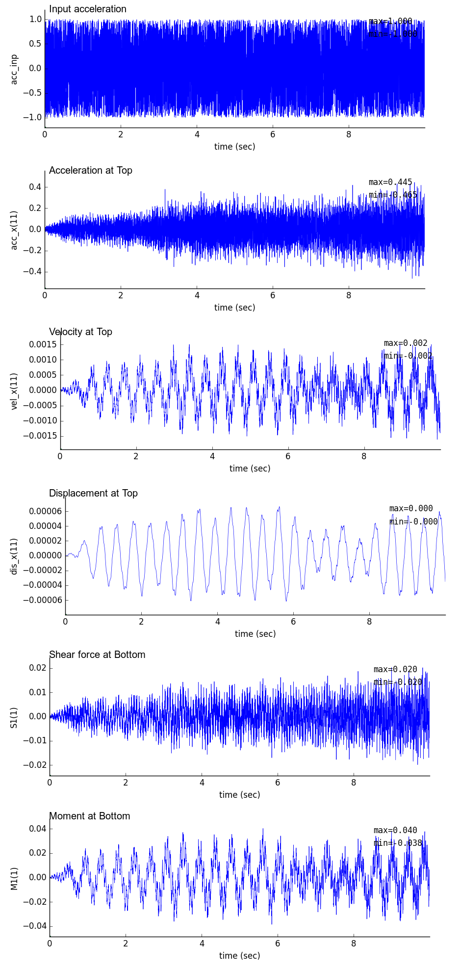
時刻歴解析出力図
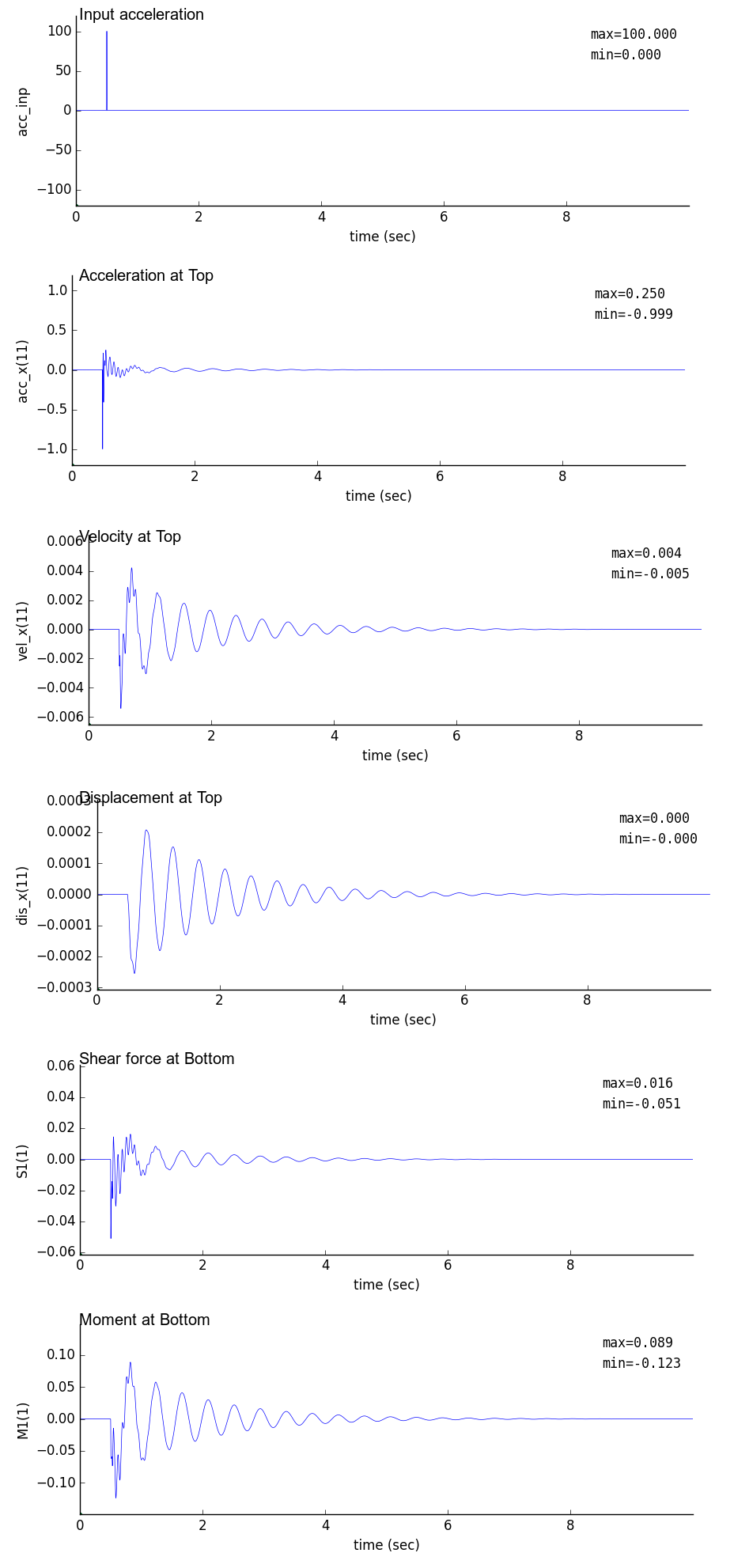
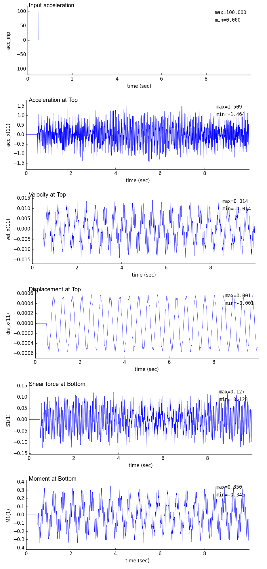
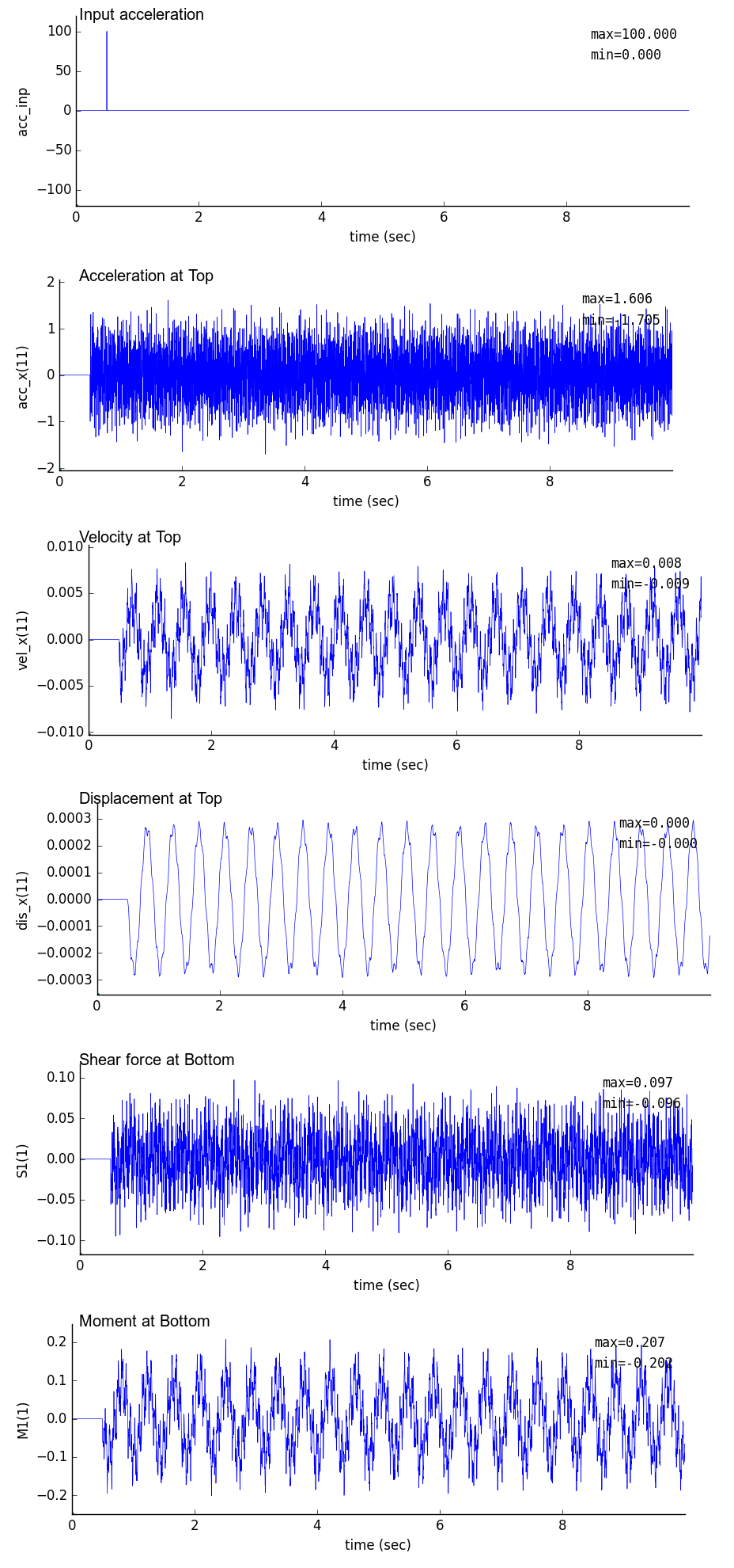
時刻0.5秒で最大100galとなるガウス波を基部に入力したときの鉛直片持梁の時刻歴解析結果を以下に示す.
解析では,時間刻み dt を 0.01,0.005,0.001 秒と変化させている.
| dt = 0.01 sec | dt = 0.005 sec | dt = 0.001 sec |
|---|
 |
 |
 |
| dt = 0.01 sec | dt = 0.005 sec | dt = 0.001 sec |
|---|
 |
 |
 |
固有振動数の比較
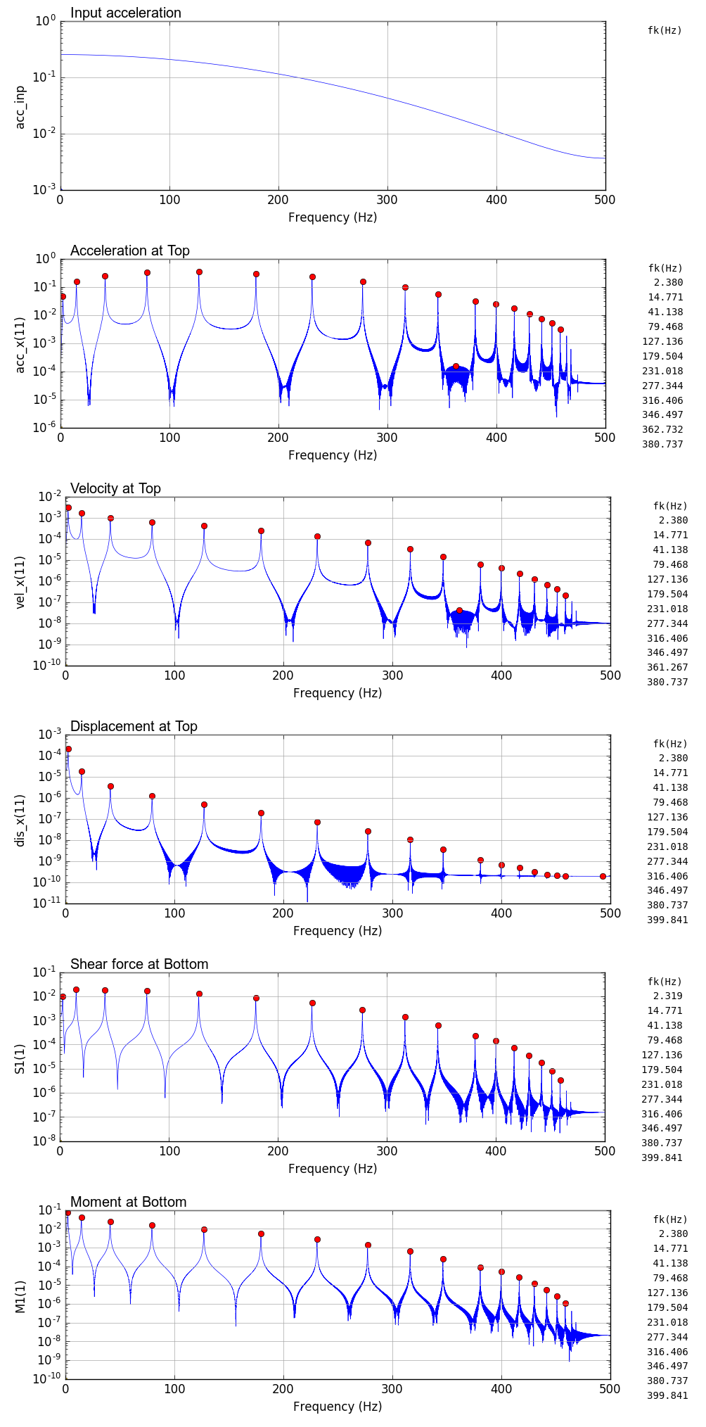
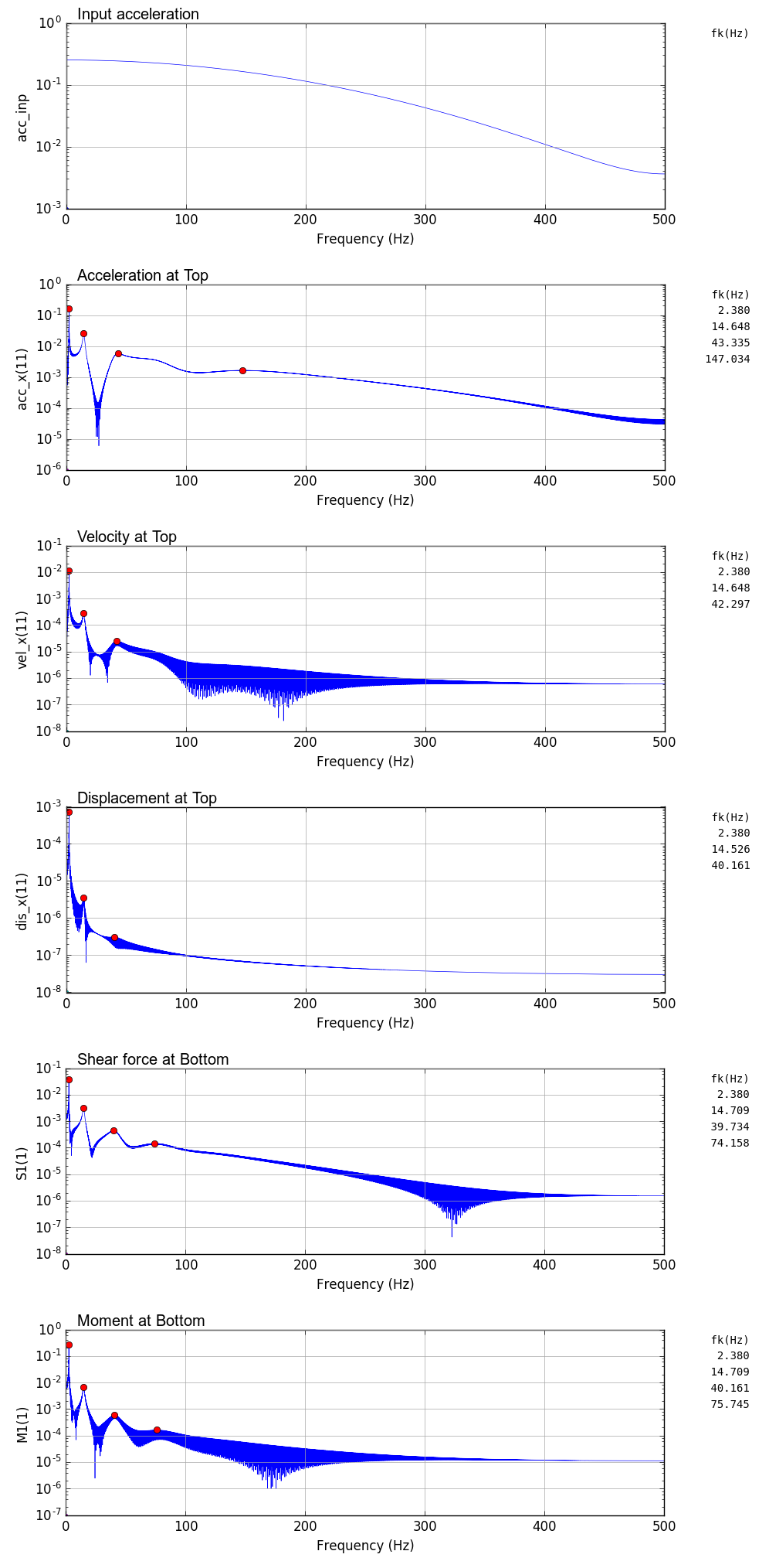
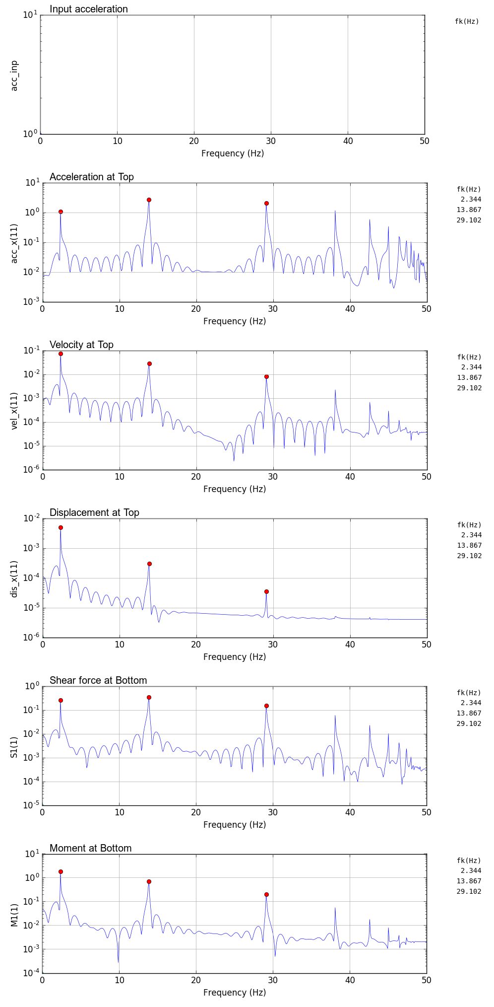
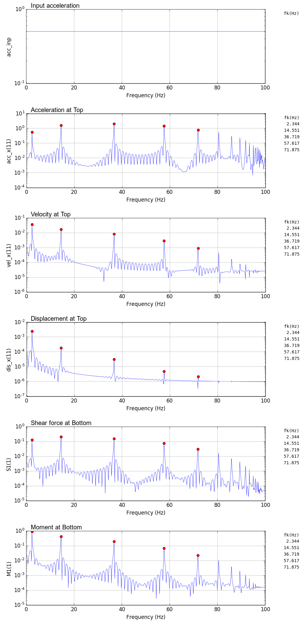
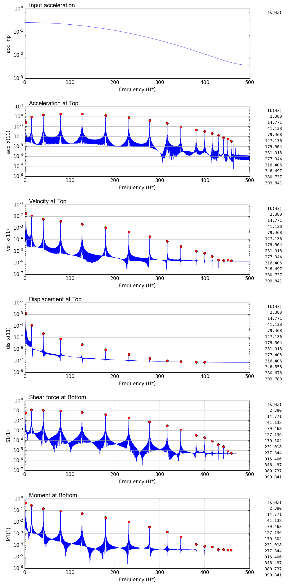
FEM解析結果のフーリエスペクトルから求めた固有振動数と理論値の比較を以下に示す.
解析結果による固有振動数は,scipy の argrelmax(sp0,order=100)でヒットしたもののみ(図中赤丸)を掲載している.解析結果では高い周波数側に検索されていないピークがあるが,高周波数側の固有振動数は誤差が大きく実際には使いものにならない.
固有振動数の比較
| 理論値 | 解析結果 |
|---|
| mode | fn(Hz) | >固有値
解析 | dt=
0.01s | dt=
0.005s | dt=
0.001s |
|---|
| 1 | 2.358 | 2.358 | 2.344 | 2.344 | 2.380 |
| 2 | 14.776 | 14.776 | 13.867 | 14.551 | 14.771 |
| 3 | 41.373 | 41.383 | 29.102 | 36.719 | 41.138 |
| 4 | 81.074 | 81.152 | | 57.617 | 79.468 |
| 5 | 134.022 | 134.359 | | 71.875 | 127.136 |
| 6 | 200.205 | 201.285 | | | 179.504 |
| 7 | 279.625 | 282.413 | | | 231.018 |
| 8 | 372.282 | 378.356 | | | 277.344 |
| 9 | 478.176 | 489.210 | | | 316.406 |
| 10 | 597.306 | 608.158 | | | 346.497 |
| 11 | 729.673 | 809.432 | | | 380.737 |
| 12 | 875.276 | 977.896 | | | 399.841 |
|
片持梁の曲げ固有振動数計算式
\begin{equation}
f_n=\cfrac{1}{2\pi}\left(\cfrac{\alpha}{\ell}\right)^2 \sqrt{\cfrac{E I}{\rho A}}
\end{equation}
$\alpha$は以下を満足する数値
\begin{equation}
\cos\alpha\cdot\cosh\alpha+1=0
\end{equation}
材料特性
$E=2,000,000 ~t/m^2$
$A=0.25 ~m^2$
$I=0.005208 ~m^4$
$\gamma=2.3 ~t/m^3$ ($\rho=\gamma~/~g~:~g=9.8m/s^2$)
$\ell=10 ~m$
|
| 固有値解析による振動モード図 |
|---|
 |
出力事例(ランダム波)
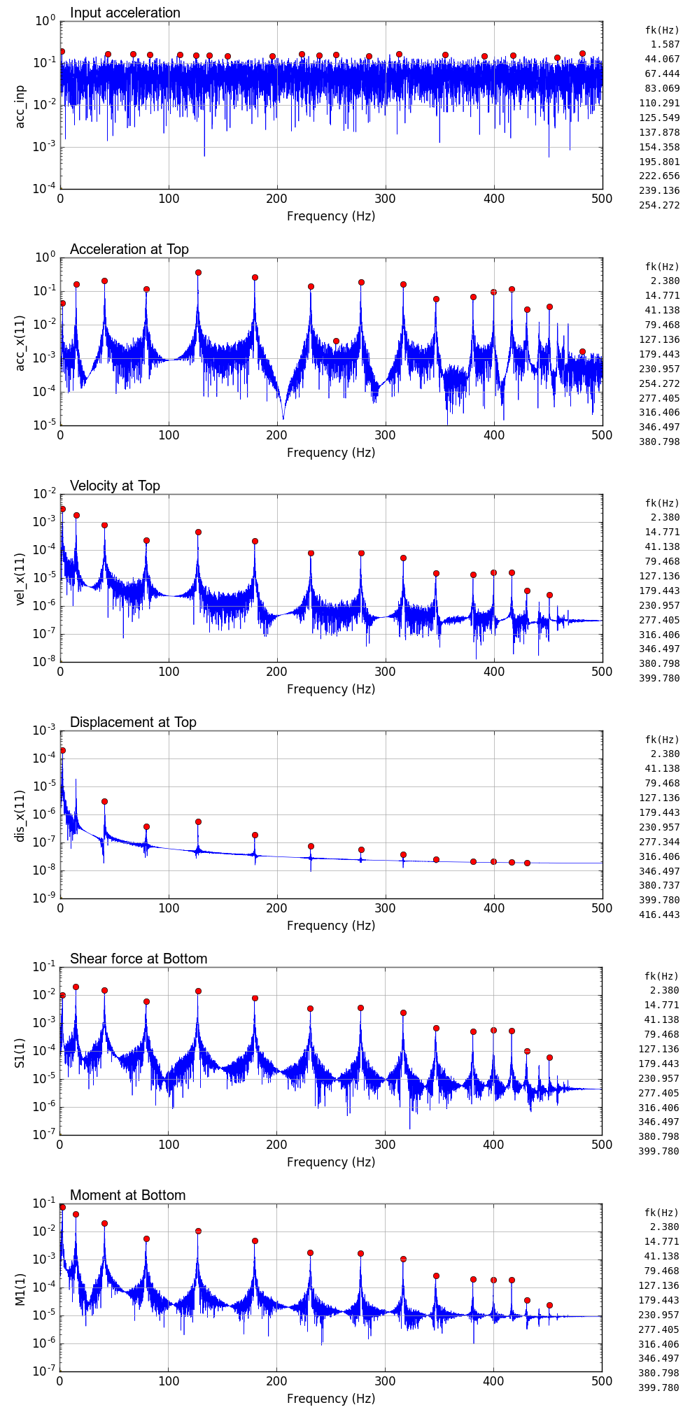
非減衰の鉛直片持梁に$\pm 1 gal$ の水平ランダム波を入力した場合の事例を示す.解析時間刻みはdt=0.001秒とした.また,scipy argrelmax による極大値検索は,order=200 として行っている:maxID=argrelmax(sp0,order=200)
| 時刻歴(dt = 0.001 sec) | フーリエスペクトル(dt = 0.001 sec) |
|---|
 |
 |
出力事例(ガウス波:減衰考慮)
時刻0.5秒で最大100galとなるガウス波を基部に入力したときの鉛直片持梁の時刻歴解析結果を示す.
以下の条件で減衰を考慮した.1次および2次の固有周期 fn は,固有値解析結果を用いた.
| Mode | fn(Hz) | h | ζ |
|---|
| 1 | 2.358 | 0.05 | ζm=1.2777 |
| 2 | 14.776 | 0.05 | ζk=0.00092888 |
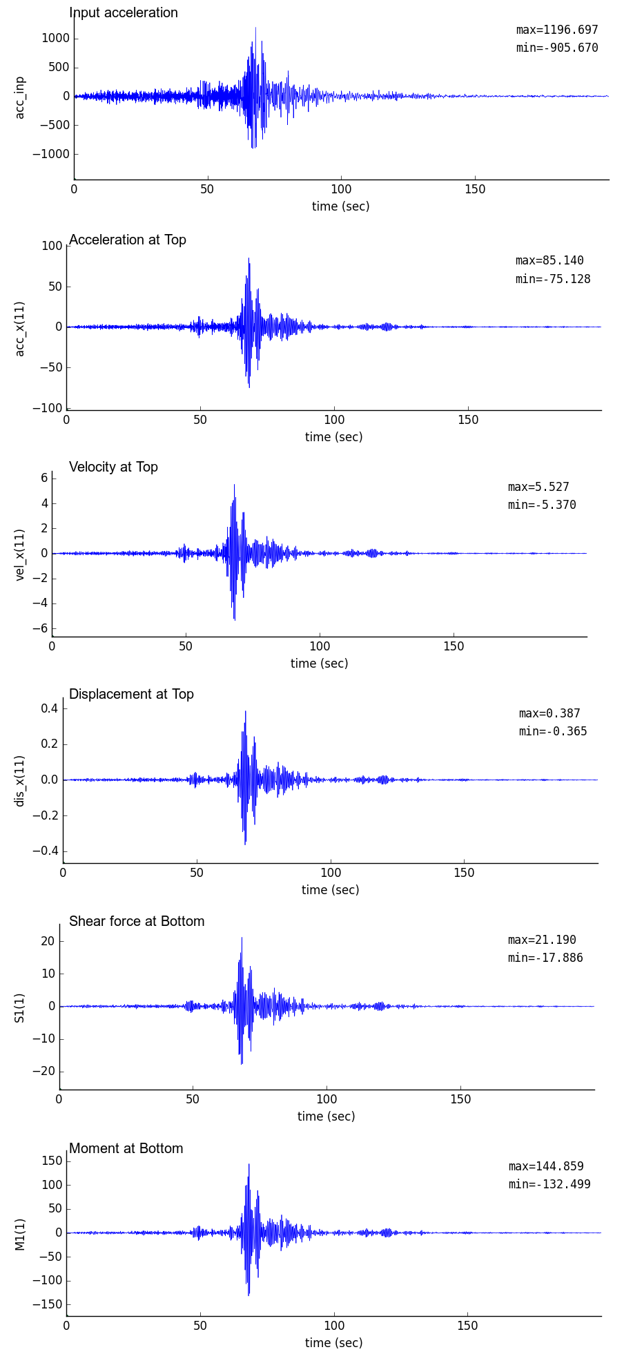
出力事例(観測地震波:減衰考慮)
減衰(ζmおよびζk)を考慮した鉛直片持梁に観測水平地震波を入力した場合の事例を示す.
減衰を示す比例定数は前項と同じ値を用いている.
解析時間刻みは,地震波のサンプリングピッチであるdt=0.01秒,およびdt=0.001秒として線形内挿したデータとした.
また,scipy argrelmax による極大値検索は,order=1000 として行っている:maxID=argrelmax(sp0,order=1000)
線形内挿のプログラムを以下に示す.scipy の interpolate を使っている.
元データは3000個あるが,用いるデータは5000から25001としている.
import numpy as np
import matplotlib.pyplot as plt
from scipy import interpolate

data = np.loadtxt("test_eq010.txt")
x0=data[5000:25001]
dt=0.01
t0=np.arange(0, 200+dt, dt)
print(len(t0), len(x0))

plt.plot(t0,x0)
plt.show()

f = interpolate.interp1d(t0, x0)
dt=0.001
t1=np.arange(0, 200, dt)
x1 = f(t1)
print(len(t1), len(x1))

plt.plot(t1,x1)
plt.show()

fout=open('inp_eq010.txt','w')
print(0.01,file=fout)
for i in range(0,len(x0)-1):
    print(x0[i],file=fout)
fout.close()

fout=open('inp_eq001.txt','w')
print(0.001,file=fout)
for i in range(0,len(x1)):
    print(x1[i],file=fout)
fout.close()
| 時刻歴(dt = 0.01 sec) | フーリエスペクトル(dt = 0.01 sec) |
|---|
 |
 |
| 時刻歴(dt = 0.001 sec) | フーリエスペクトル(dt = 0.001 sec) |
|---|
 |
 |
2次元弾性骨組構造幾何学的非線形解析
プログラム概要
- このプログラムは,要素微小変位の仮定において2次元弾性平面骨組の幾何学的非線形解析を行うものである.
- 要素として,1要素2節点,1節点3自由度(水平変位・鉛直変位・回転)を有する梁要素が用いられている.
- 荷重として,節点外力増分のみを扱える.
- 釣り合い条件を求めるための解析手法として,弧長法を用いている.これにより変位は増大するが荷重が減少するような現象も追跡できる.
- 座標システムにおいては,右方向をx軸,上方向をy軸,反時計回りを正の回転方向と設定している.
- 連立一次方程式は,numpy.linalg.solve(A, b) で解いている.
- 入力データファイル,出力データファイルは,空白区切りで記載される必要があり,ファイル名はコマンドライン引数として入力する.
| 扱える境界条件 |
|---|
| 項目 | 説明 |
|---|
| 節点外力増分 | 載荷節点数,載荷節点番号,荷重増分値を指定 |
| 節点変位拘束 | 変位拘束節点数,拘束節点番号を指定(完全拘束:変位=0のみ扱える) |
FEM解析プログラム
FEM解析実行用スクリプト
python3 py_fem_gfrmAL.py inp.txt out.txt nnmax
| inp.txt | : 入力データファイル(空白区切りデータ) |
| out.txt | : 出力データファイル(空白区切りデータ) |
| nnmax | : 載荷ステップ数 |
入力データ書式
npoin  nele  nsec  npfix  nlod  # Basic values for analysis
E  A  I                         # Material properties
    ..... (1 to nsec) .....     #
node_1  node_2  isec            # Element connectivity, material set number
    ..... (1 to nele) .....     #
x  y                            # Node coordinate of node
    ..... (1 to npoin) .....    #
lp  fix_x  fix_y  fix_r         # Restricted node number
    ..... (1 to npfix) .....    #
lp  df_x  df_y  df_r            # Loaded node and loading conditions (load increment)
    ..... (1 to nlod) .....     #     (omit data input if nlod=0)
| npoin, nele, nsec | : 節点数,要素数,断面特性数 |
| npfix, nlod | : 拘束節点数,載荷節点数 |
| E, A, I | : 弾性係数,断面積,断面2次モーメント |
| node_1, node_2, isec | : 節点1,節点2,断面特性番号 |
| x, y | : x座標,y座標 |
| lp, fix_x, fix_y, fix_r | : 節点番号,x・y・回転方向の拘束の有無(0: 自由,1: 完全拘束) |
| lp, df_x, df_y, df_r | : 節点番号,x・y・回転方向荷重 |
出力データ書式
npoin  nele  nsec npfix  nlod  nnmax
    (Each value of above)
sec  E  A  I
    sec   : Material number
    E     : Elastic modulus
    A     : Section area
    I     : Moment of inertia
    ..... (1 to nsec) .....
node  x  y  fx  fy  fr  kox  koy  kor
    node   : Node number
    x      : x-coordinate
    y      : y-coordinate
    fx     : Load in x-direction
    fy     : Load in y-direction
    fr     : Moment load
    kox    : Index of restriction in x-direction (0: free, 1: fixed)
    koy    : Index of restriction in y-direction (0: free, 1: fixed)
    kor    : Index of restriction in rotation    (0: free, 1: fixed)
    ..... (1 to npoin) .....
elem  i  j  sec
    elem : Element number
    i    : Node number of start point
    j    : Node number of end point
    sec  : Material number
    ..... (1 to nele) .....
* nnn=0 iii=0 lam=0.0
node  fp-x  fp-y  fp-r  dis-x  dis-y  dis-r  dr-x  dr-y dr-r
    node  : Node number
    fp-x  : Total load in x-direction
    fp-y  : Total load in y-direction
    fp-r  : Total load in rotation
    dis-x : Displacement in x-direction
    dis-y : Displacement in y-direction
    dis-r : Displacement in rotation
    dr-x  : Un-balanced force in x-direction
    dr-y  : Un-balanced force in y-direction
    dr-r  : Un-balanced force in rotation
    ..... (1 to npoin) .....
elem  N_i  S_i  M_i  N_j  S_j  M_j
    elem : Element number
    N_i  : Axial force of node-i
    S_i  : Shear force of node-i
    M_i  : Moment of node-i
    N_j  : Axial force of node-j
    S_j  : Shear force of node-j
    M_j  : Moment of node-j
    ..... (1 to nele) .....
* nnn=1 iii=xx lam=xxx
node  fp-x  fp-y  fp-r  dis-x  dis-y  dis-r  dr-x  dr-y dr-r
    node  : Node number
    fp-x  : Total load in x-direction
    fp-y  : Total load in y-direction
    fp-r  : Total load in rotation
    dis-x : Displacement in x-direction
    dis-y : Displacement in y-direction
    dis-r : Displacement in rotation
    dr-x  : Un-balanced force in x-direction
    dr-y  : Un-balanced force in y-direction
    dr-r  : Un-balanced force in rotation
    ..... (1 to npoin) .....
elem  N_i  S_i  M_i  N_j  S_j  M_j
    elem : Element number
    N_i  : Axial force of node-i
    S_i  : Shear force of node-i
    M_i  : Moment of node-i
    N_j  : Axial force of node-j
    S_j  : Shear force of node-j
    M_j  : Moment of node-j
    ..... (1 to nele) .....

.... .... ....

* nnn=nnmax-1 iii=xx lam=xxx
node  fp-x  fp-y  fp-r  dis-x  dis-y  dis-r  dr-x  dr-y dr-r
    ..... (1 to npoin) .....
elem  N_i  S_i  M_i  N_j  S_j  M_j
    ..... (1 to nele) .....
n=(total degrees of freedom)  time=(calculation time)
| fp-x, fp-y, fp-r | : x方向荷重,y方向荷重,回転方向荷重 |
| dis-x, dis-y, dis-r | : x方向変位,y方向変位,回転変位 |
| dr-x, dr-y, dr-r | : x方向不平衡力,y方向不平衡力,回転方向不平衡力 |
| N, S, M | : 軸力,せん断力,モーメント |
| n | : 全自由度(連立方程式の元) |
| time | : 計算時間 |
出力事例
荷重-変位曲線作図プログラム py_fig_gfrm.py
荷重変位曲線作成プログラム py_fig_gfrm.py では,汎用性を出そうとした結果,コマンドラインからの入力がかなりごたつくことになってしまった.
変位モード図作成プログラム py_fig_gfrm_mode.py
変位モード図作成プログラム py_fig_gfrm_mode.py では,変位モードのみでは汎用性のあるものを比較的平易に実現できるが,境界条件を入れようとするとかなり複雑になってしまう.よって,作成したいグラフは4枚のみなので,プログラム内で入力ファイルを指定し,ファイル毎に個別の処理をしている.
(荷重を示す矢印)
荷重を示す矢印は,arrowで書いている.arrowでは
ax.arrow(x,y,u,v,head_length=hl, ....)
のような命令を書き込んでいる.
例えば鉛直の矢印を描く場合,矢印の尻尾から先端までの長さは,( v + head_length ) となることに注意して扱う必要がある.実際の対応は以下の通り.
uu=0.0
vv=(ymax-ymin)*0.1
x1=xx[lnod-1]
y1=yy[lnod-1]+vv
hl=vv*0.4
hw=hl*0.5
ax.arrow(x1,y1,uu,-(vv-hl), lw=2.0,head_width=hw, head_length=hl, fc='#555555', ec='#555555')
(固定端を示す記号)
鉛直片道梁の基部に描いている固定端を示す記号は,fill(... hatch='///') を使って描いている.
ここで,fillでは長方形領域を指定しているが,枠線は不要なので,fill の中で,linewidth=0.0 を指定して枠線を描画しないようにしている.実際の対応は以下の通り.
lp=1; x1=x[lp-1]; y1=y[lp-1]
px=[x1-2*scl,x1+2*scl,x1+2*scl,x1-2*scl]
py=[y1,y1,y1-1*scl,y1-1*scl]
ax.fill(px,py,fill=False,linewidth=0.0,hatch='///')
ax.plot([x1-2*scl,x1+2*scl],[y1,y1],color='#000000',linestyle='-',linewidth=1.5)
FEM計算実行・荷重変位曲線作図プログラム実行用スクリプト
# FEM calculation by Arc-Length method
python py_fem_gfrmAL.py inp_gfrm_canti.txt out_gfrm_canti.txt 70
python py_fem_gfrmAL.py inp_gfrm_cable.txt out_gfrm_cable.txt 290
python py_fem_gfrmAL.py inp_gfrm_arch.txt out_gfrm_arch.txt 310
python py_fem_gfrmAL.py inp_gfrm_lee.txt out_gfrm_lee.txt 160

# Drawing of Load-displacement curve
python py_fig_gfrm.py out_gfrm_canti.txt 11 11 -411.07 1000 1000 \$u/L\$ $\v/L\$ \$u/L\$\,$\v/L\$ \$P/P_{cr}\$ LL
python py_fig_gfrm.py out_gfrm_cable.txt 12 11 -1644.3 1000 1000 \$u/L\$ \$v/L\$ \$u/L\$\,\$v/L\$ \$P/P_{cr}\$ LL
python py_fig_gfrm.py out_gfrm_arch.txt 21 21 -666.4 -500 -500 \$u/R\$ \$v/R\$ \$u/R\$\,\$v/R\$ \$P\\cdot\(R^2/EI\)\$ UL
python py_fig_gfrm.py out_gfrm_lee.txt 13 13 -166.6 1000 -1000 \$u/L\$ \$v/L\$ \$u/L\$\,\$v/L\$ \$P\\cdot\(L^2/EI\)\$ LL

# Drawing of displacement mode
python py_fig_gfrm_mode.py
python py_fig_gfrm.py out.txt node-L node-D nd-L nd-u nd-v leg-u leg-v x-Label y-Label loc
| out.txt | :FEM出力データファイル(空白区切りデータ) |
| node-L | :荷重変位曲線を描くための載荷節点番号 |
| node-D | :荷重変位曲線を描くための変位描画節点番号 |
| nd-L | :荷重無次元化のための数値(符号含む) |
| nd-u | :x方向変位無次元化のための数値(符号含む) |
| nd-v | :y方向変位無次元化のための数値(符号含む) |
| leg-u | :x方向変位ラベル(凡例用) |
| leg-v | :y方向変位ラベル(凡例用) |
| x-Label | :x軸ラベル(Displacement) |
| y-Label | :y軸ラベル(Load) |
| loc | :凡例描画位置 |
変位モードおよび荷重-変位曲線出力事例
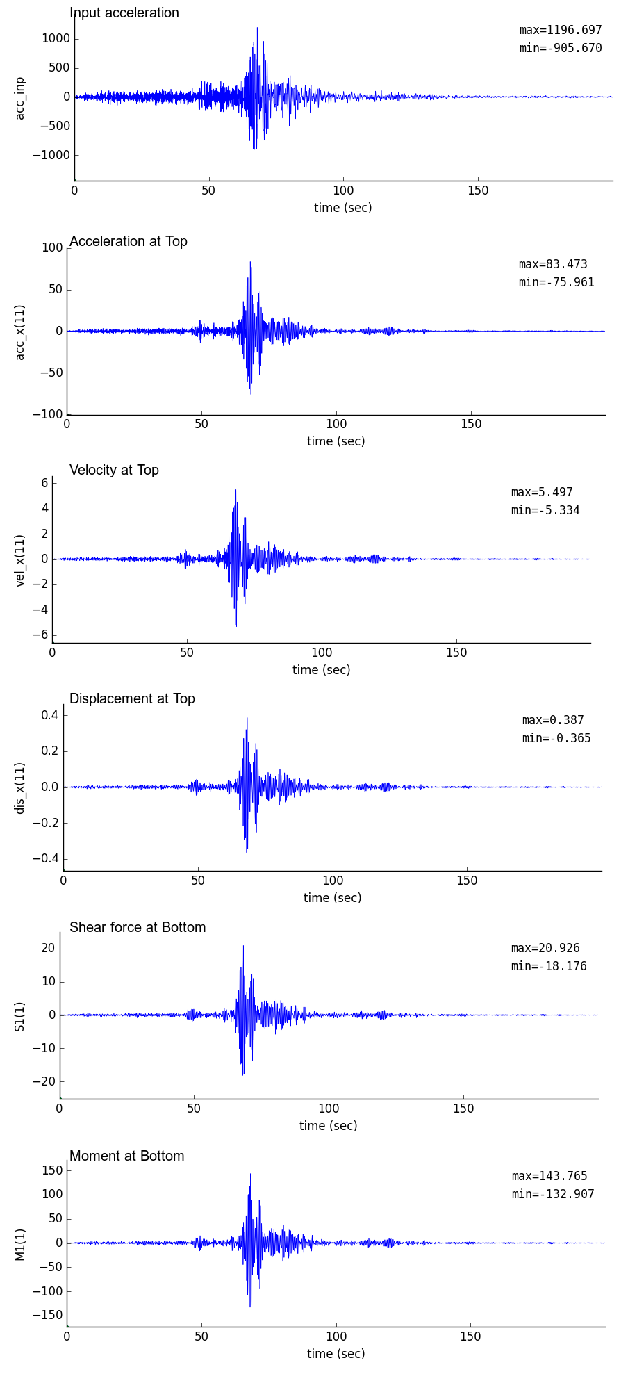
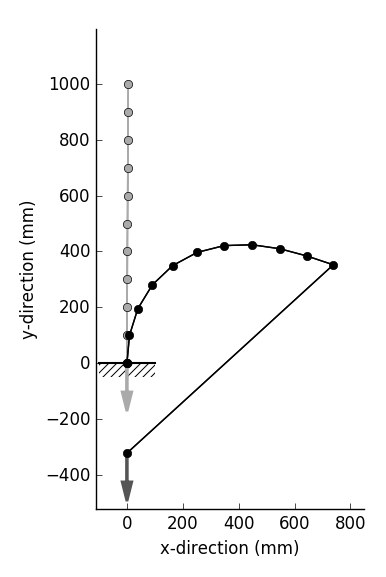
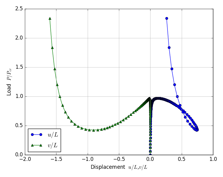
| 軸圧縮力を受ける片持梁(inp_gfrm_canti.txt) |
|---|
L=1,000mm, E=200,000MPa, A=100m$^2$, I=833m$^4$
Initial deflection $v_0$=1mm
Buckling load $P_{cr}=\pi^2 EI / 4 L^2$=411.07N |
| Displacement mode | Displacements at Top |
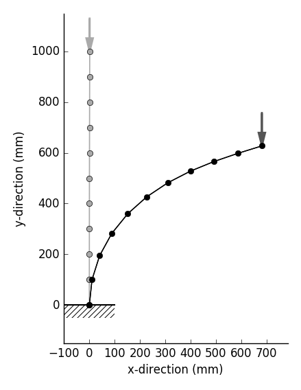 |
 |
| ケーブルで先端を引っ張られる片持梁(inp_gfrm_cable.txt) |
|---|
Column: L=1,000mm, E=200,000MPa, A=100m$^2$, I=833m$^4$
Cable: L=1,000mm, E=200,000MPa, A=28.3$^2$
Initial deflection $v_0$=5mm
Buckling load $P_{cr}=\pi^2 EI / L^2$=1644.3NN |
| Displacement mode | Displacements at Top |
 |
 |
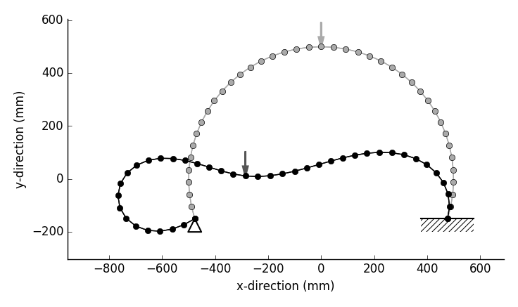
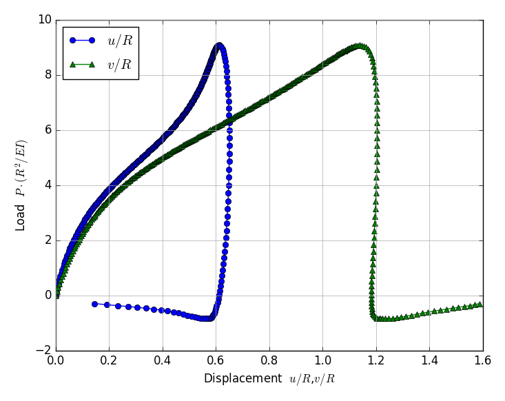
| 鉛直集中荷重を受ける非対称支持されたアーチ(inp_gfrm_arch.txt) |
|---|
| R=500mm, Center angle=215$^\circ$, E=200,000MPa, A=100m$^2$, I=833m$^4$ |
| Displacement mode | Displacements at Loading point |
 |
 |
| 鉛直集中荷重を受けるフレーム(inp_gfrm_lee.txt) |
|---|
| L=1000mm, E=200,000MPa, A=100m$^2$, I=833m$^4$ |
| Displacement mode | Displacements at Loading point |
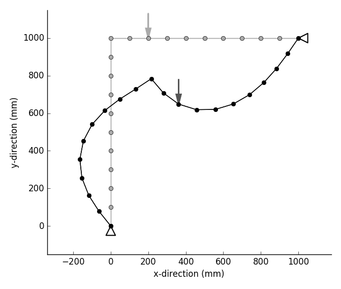 |
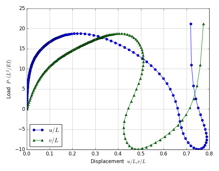 |
2次元弾性骨組座屈解析
プログラム概要
- このプログラムは,2次元弾性平面骨組の線形座屈解析を行うものである.
- 荷重の方向は,座屈変形後も変わらない条件となっている.
- 要素として,1要素2節点,1節点3自由度(水平変位・鉛直変位・回転)を有する梁要素が用いられている.
- 座標システムにおいては,右方向をx軸,上方向をy軸,反時計回りを正の回転方向と設定している.
- 固有値解析を行う前に,入力した荷重を用いて線形解析を1回行い,固有値解析用マトリックスの初期軸力を設定している.固有値は係数として算定されるため,実際の座屈荷重は,初期軸力に固有値を乗じたものになる.
- 固有値解析時の軸力は,圧縮を正とする.
- 固有方程式は,w,vr=scipy.linalg.eig(K, G) を用い一般化固有値問題として解いている.
- 入力データファイル,出力データファイルは,空白区切りで記載される必要があり,ファイル名はコマンドライン引数として入力する.
| 扱える境界条件 |
|---|
| 項目 | 説明 |
|---|
| 節点外力 | 載荷節点数,載荷節点番号,荷重増分値を指定 |
| 節点変位拘束 | 変位拘束節点数,拘束節点番号を指定(完全拘束:変位=0のみ扱える) |
FEM解析プログラム
FEM解析実行用スクリプト
python3 py_fem_bfrm.py inp.txt out.txt
| inp.txt | : 入力データファイル(空白区切りデータ) |
| out.txt | : 出力データファイル(空白区切りデータ) |
入力データ書式
npoin  nele  nsec  npfix  nlod  # Basic values for analysis
E  A  I                         # Material properties
    ..... (1 to nsec) .....     #
node_1  node_2  isec            # Element connectivity, material set number
    ..... (1 to nele) .....     #
x  y                            # Node coordinate of node
    ..... (1 to npoin) .....    #
lp  fix_x  fix_y  fix_r         # Restricted node number
    ..... (1 to npfix) .....    #
lp  df_x  df_y  df_r            # Loaded node and loading conditions (load increment)
    ..... (1 to nlod) .....     #     (omit data input if nlod=0)
| npoin, nele, nsec | : 節点数,要素数,断面特性数 |
| npfix, nlod | : 拘束節点数,載荷節点数 |
| E, A, I | : 弾性係数,断面積,断面2次モーメント |
| node_1, node_2, isec | : 節点1,節点2,断面特性番号 |
| x, y | : x座標,y座標 |
| lp, fix_x, fix_y, fix_r | : 節点番号,x・y・回転方向の拘束の有無(0: 自由,1: 完全拘束) |
| lp, df_x, df_y, df_r | : 節点番号,x・y・回転方向荷重 |
出力データ書式
npoin  nele  nsec npfix  nlod
    (Each value of above)
sec  E  A  I
    sec   : Material number
    E     : Elastic modulus
    A     : Section area
    I     : Moment of inertia
    ..... (1 to nsec) .....
node  x  y  fx  fy  fr  kox  koy  kor
    node   : Node number
    x      : x-coordinate
    y      : y-coordinate
    fx     : Load in x-direction
    fy     : Load in y-direction
    fr     : Moment load
    kox    : Index of restriction in x-direction (0: free, 1: fixed)
    koy    : Index of restriction in y-direction (0: free, 1: fixed)
    kor    : Index of restriction in rotation    (0: free, 1: fixed)
    ..... (1 to npoin) .....
elem  i  j  sec
    elem : Element number
    i    : Node number of start point
    j    : Node number of end point
    sec  : Material number
    ..... (1 to nele) .....
Order         1       2       3  ......
lambda     w[1]   w[2]    w[3]  ......
v[  1]   v[1,1]  v[1,2]  v[1,3]  ......
v[  2]   v[1,1]  v[1,2]  v[1,3]  ......
......   ......  ......  ......  ......
v[  n]   v[1,1]  v[1,2]  v[1,3]  ......
    Order   : Ranking
    w[i]    : Buckling coefficient (eigen value)
    v[j,i]  : Element of eigen vector
n=(total degrees of freedom)  time=(calculation time)
| fx, fy, fr | : x方向荷重,y方向荷重,回転方向荷重 |
| w[i] | : 固有値(昇順) |
| v[j,i] | : 固有ベクトル(変位モードを示す) |
| n | : 全自由度(連立方程式の元) |
| time | : 計算時間 |
出力事例
FEM計算実行・座屈変形モード図作成プログラム実行用スクリプト
固有値解析・座屈変形モード図作成プログラム実行後,ImageMagick の convert コマンドにより画像の結合を行っている.
python py_fem_bfrm.py inp_circ.txt out_circ.txt
python py_fig_bfrm_mode.py out_circ.txt

convert +append fig_0.png fig_1.png fig_2.png _1.png
convert +append fig_3.png fig_4.png fig_5.png _2.png
convert +append fig_6.png fig_7.png fig_8.png _3.png
convert +append fig_9.png fig_10.png fig_11.png _4.png
convert -append _1.png _2.png _3.png _4.png fig_bmode.png
座屈モード出力事例
計算条件
円環直径:3,000mm,板厚:20mm,奥行き:1mm,弾性係数:200,000MPa, 初期水圧:1MPa
節点数:180,要素数:180
理論座屈荷重計算式
「座屈時も外圧の方向は変わらない」場合の円環の座屈荷重は次式で計算している.
\begin{equation}
P_{cr}=\cfrac{n^2 E I}{R^3} \qquad (n=2, 3, 4, ......)
\end{equation}
理論値計算には,E=200,000MPa, I=666.666mm^4, R=1500mm を使用している.
理論値と固有値解析結果の比較
| モード(n) | 2 | 3 | 4 | 5 | 6 | 7 | 8 |
|---|
| 理論座屈圧力(MPa) | 0.158 | 0.356 | 0.632 | 0.988 | 1.422 | 1.936 | 2.528 |
|---|
| 計算座屈圧力(MPa) | 0.158 | 0.356
0.356 | 0.627
0.632 | 0.988
0.988 | 1.413
1.423 | 1.936
1.936 | 2.528 |
|---|
| 外水圧を受ける円環の座屈モード |
|---|
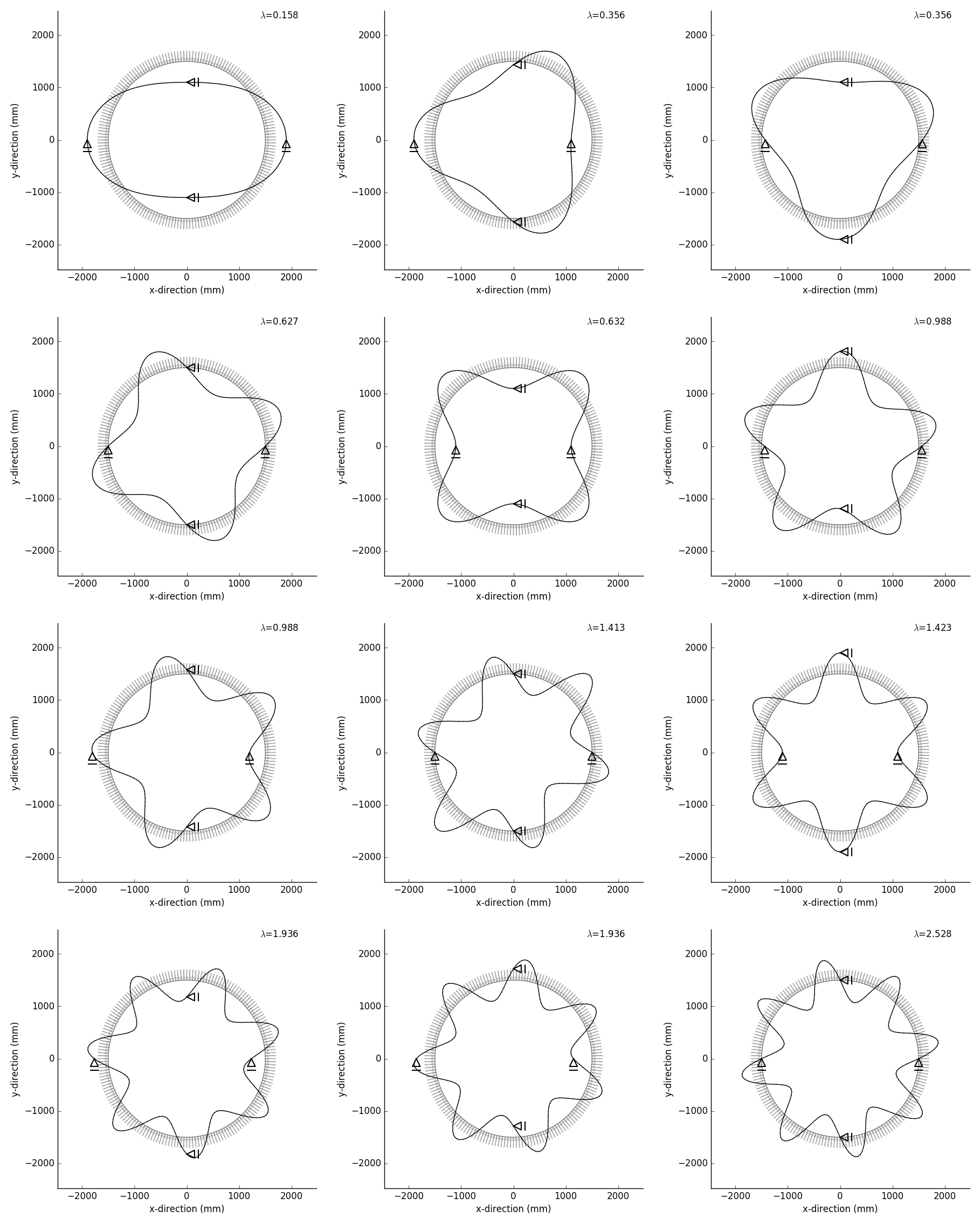 |
1次元非定常熱伝導解析
プログラム概要
- このプログラムは,1次元非定常熱伝導解析を行うものである.定常熱伝導問題には対応していない.
- 1次元ではあるが,コンクリートの打継(複数リフトの打設)を,打設時刻とその時点で有効な要素を指定することにより.自動的に考慮できる.
- 座標系においては,x方向を上向きと仮定している
- 1次元解析なので,要素側面は全て断熱条件であり,領域の下面と上面のみ,境界条件が考慮できる.
- 領域上下面の境界条件として,断熱境界,熱伝達境界が考慮できる.
- セメント・コンクリートをモデルとした発熱体を扱うことができる.
- 要素として,1要素2節点,1節点1自由度(温度あるいは熱流束)を有する線形要素が用いられている.
- 時間軸の離散化には,Crank-Nicolson 法が用いられている.
- 連立一次方程式は,numpy.linalg.inv(A) でリフト打設毎(要素数が増えるごと)に1回逆行列を求めこれを記憶して温度履歴を求めている.
- 入力データファイル,出力データファイルは,空白区切りで記載される必要があり,ファイル名はコマンドライン引数として入力する.
- 入力データファイルには,モデル領域を定義するものと,熱伝達境界外部温度の履歴を定義するものの,2種類が必要である.
- 出力事例でも示すが,このプログラムでは,要素分割を細かくしないと精度は出ない.
| 扱える境界条件 |
|---|
| 項目 | 説明 |
|---|
| 断熱境界 | モデル領域の定義ファイルでモデル下端および上端の条件を指定する. |
| 熱伝達境界 | モデル領域の定義フィルで熱伝達率を指定する.また別ファイルでモデル下端および上端の熱伝達境界の外部温度履歴を指定する. |
温度指定境界について
このプログラムでは,温度指定境界は扱えない.温度固定の条件で連立方程式を処理して計算を試みたが,予想に反する答えしか出てこず,改善策が見つかっていない.
しかしながら,工学的には,大きな熱伝達率を入力し外部温度を設定すれば,近似的に温度固定境界と同等の条件を再現することがでる.
FEM解析プログラム
FEM解析実行用スクリプト
python py_fem_1Dheat.py inp1.txt inp2.txt out.txt
| inp1.txt | : 解析モデルデータ入力ファイル(空白区切りデータ) |
| inp2.txt | : 熱伝達境界外部温度の履歴入力ファイル(空白区切りデータ) |
| out.txt | : 出力データファイル(空白区切りデータ) |
入力データ書式
解析モデルデータ
npoin  nele  nsec  koB  koT  delta  nlift  # Basic values for analysis
Ak  Ac  Arho  Tk  Al  AA                   # Material properties
     ..... (1 to nsec) .....               #
tlift_1  tlift_2  .... (1 line input) .... # Placing time of each lift
alphac_B  alphac_T                         # Heat transfer rates of bottom and top
node-1  node-2  isec  lift                 # Element connectivity, Material set number, lift number
     ..... (1 to nele) .....               #   (counterclockwise order of node numbers)
x  T0                                      # Coordinates of node, initial temperature of node
     ..... (1 to npoin) .....              #
n1out                                 # Number of nodes for output of temperature time history
n1node_1  ..... (1 line input) .....  # Node number for above
n2out                                 # frequency of output of temperatures of all nodes
n2step_1  ..... (1 line input) .....  # Time step number for above (Omit data input if ntout=0)
| npoin, nele, nsec | : 節点数,要素数,材料特性数 |
| koB | : 下端境界条件(0:断熱,1:熱伝達) |
| koT | : 上端境界条件(0:断熱,1:熱伝達) |
| delta | : 計算時間間隔 |
| nlift | : 打設リフト数 |
| Ak, Ac, Arho | : 熱伝導率,比熱,密度 |
| Tk, Al, AA | : 最高断熱上昇温度,発熱速度パラメータ,要素断面積 |
| x, T0 | : 節点座標,節点初期温度 |
| n1out | : 全時刻歴を出力する節点数 |
| n1node | : 全時刻歴を出力する節点番号 |
| n2out | : 全節点温度を出力する時間ステップ数 |
| n2step | : 全節点温度を出力する時間ステップ番号 |
熱伝達境界外部温度の履歴
空白区切りで,3列の数値の入力が必須である.たとえ熱伝達境界でなくても0などの適当な数値を入力しておく必要がある.
 0   TcinB[0]  TcinT[0]
 1   TcinB[1]  TcinT[1]
 2   TcinB[2]  TcinT[2]
 ..  ........  ........
 i   TcinB[i]  TcinT[i]
 ..  ........  ........
 .... (until end of calculation time) ....
| TcinB | : 下端熱伝達境界外部温度履歴 |
| TcinT | : 上端熱伝達境界外部温度履歴 |
出力データ書式
npoin  nele  nsec  koB  koT  delta  nlift  niii  n1out  n2out
    (Each value of above)
sec  Ak  Ac  Arho  Tk  Al  AA
    sec  : Material number
    Ak   : Heat conductivity coefficient
    Ac   : Specific heat
    Arho : Unit weight
    Tk   : Maximum temperature rize
    Al   : Heat release rate
    AA   : Section area of element
    ..... (1 to nsec) .....
node  x  tempe0  alphac
    node   : Node number
    x      : x-ccordinate
    tempe0 : Initial temperature
    alphac : Heat transfer rate of bottom and top node
    ..... (1 to npoin) .....
elem  i  j  sec  lift  time
    elem : Element number
    i    : Node number of start point
    j    : Node number of second point
    sec  : Material number
    lift : Lift number
    time : Placing time of lift
    ..... (1 to nele) .....
iii  ttime  Node_(xx)  Node_(xx)  Node_(xx) .....
    iii       : Time step
    ttime     : Time
    Node-(xx) : Node number
    Time historis of each node temperature are written.
    ..... (0 to end of calculation time) .....
node  t=0.0  t=(xx)  t=(xx)0  t=(xx) .....
    node   : Node number
    t=(xx) : Specified time
    Node temperatures at specified time are written.
    ..... (1 to npoin) .....
n=(total degrees of freedom)  time=(calculation time)
出力事例
モデル概要
高さ10mの既設のコンクリートブロックの上に,1リフト高2mのコンクリートを5リフト打ち上げた場合の温度履歴を計算する.既設コンクリートは発熱は終わっており,初期温度は下端で10度,表面で20度に設定している.新規打設コンクリートは,打設温度30度でリフト表面は熱伝達境界(熱伝達率10 kcal/m$^2$ h $^{\circ}$C)とし,外部温度は20度に設定している.
既設コンクリート下端は,近似的に温度固定境界とするため,熱伝達率を10000 kcal/m$^2$ h $^{\circ}$Cと大きくとっている.
| Characteristics of model |
|---|
| Heat conductivity coefficient | 2.5 kcal/m h $^{\circ}$C |
| Specific heat | 0.28 kcal/kg $^{\circ}$C |
| Unit weight | 2350 kg/m$^3$ |
Adiabatic temperature raise
for new concrete | $T=K\cdot(1-e^{-\alpha t})$, K=40$^{\circ}$C, α=0.2, t: hour |
| Element section area | 1m$^2$ |
| Model | Total length: 20m
Old concrete: 10m
New concrete: 10m,
5 lifts with height of 2m, Placing interval: 3 days (72 hours) |
| Conditions for analysis |
|---|
| New concrete placing temperature | 30 $^{\circ}$C |
| Old concrete initial temperature | from 10 $^{\circ}$C at bottom to 20 $^{\circ}$C at surface |
| Boundary condition of bottom | Temperature fixed with outside temperature 10 $^{\circ}$c (approximately)
Heat transfer rate of bottom boundary: 10000 kcal/m$^2$ h $^{\circ}$C
|
| Boundary condition of top | Heat transfer boundary with outside temperature of 20 $^{\circ}$C
Heat transfer rate of top boundary: 10 kcal/m$^2$ h $^{\circ}$C |
| Time increment for analysis | 0.1 hour |
FEM解析実行用スクリプト
python py_fem_1Dheat.py inp_100L1.txt inp_2L2.txt out_100L.txt
python py_fem_1Dheat.py inp_40L1.txt inp_2L2.txt out_40L.txt
python py_fem_1Dheat.py inp_20L1.txt inp_2L2.txt out_20L.txt
| inp_100L1.txt | : 解析モデルデータ入力ファイル(空白区切りデータ,100要素) |
| inp_40L1.txt | : 解析モデルデータ入力ファイル(空白区切りデータ,40要素) |
| inp_20L1.txt | : 解析モデルデータ入力ファイル(空白区切りデータ,20要素) |
| inp_2L2.txt | : 熱伝達境界外部温度の履歴入力ファイル(空白区切りデータ) |
| out_1D.txt | : FEM解析出力データファイル(空白区切りデータ) |
温度履歴作図プログラム実行用スクリプト
python py_fig_1Dheat.py out_100L.txt
cp _fig_tem_his.png fig_his_100.png

python py_fig_1Dheat.py out_40L.txt
cp _fig_tem_his.png fig_his_040.png

python py_fig_1Dheat.py out_20L.txt
cp _fig_tem_his.png fig_his_020.png
このプログラムでは,_fig_tem_his.png という画像ファイルが自動的に作成される.
節点温度履歴図出力事例
プログラム:py_fig_1Dheat.py を用い matplotlib で作成した png 画像を示す.
要素分割数は 20,40,100 の3ケースとしている.
要素分割20では何かがおかしい!赤い楕円で囲まれた部分に着目してみると,以下のことに気が付くと思う.
- 打設温度30度,断熱温度上昇量40度のコンクリートなのに最高温度が75度以上まで上がっている.
- 新コンクリートとの境界付近の旧コンクリートにおいて,1リフト打設直後にあり得ない温度履歴となっている.
上記現象は,要素数の増加に伴い改善されていることがわかる.