Contents
Rectangular Domain Meshing
1. Outline
This program has been made to contribute the creating test data with 4 nodes element.
Number of nodes, number of elements, element-node relationships and node coordinate are established by inputting the dimensions of rectangular domain and division number of each side. THe model drawing is also created to confirm the generated mesh data.
Following site is very useful for the treatment of 'matplotlib paches'.
http://matthiaseisen.com/matplotlib/
2. Program for rectangular domain meshing
| Program name | Description |
|---|
| py_rectmesh.py | Program for rectangular domain meshing |
3. Command format for execution
python py_rectmesh.py aa bb nn mm x0 y0 > out.txt
| aa | : length of domain in x-direction |
| bb | : length of domain in y-direction |
| nn | : division number of domain in x-direction |
| mm | : division number of domain in y-direction |
| x0 | : x-coordinate of left-bottom of domain |
| y0 | : y-coordinate of left-bottom of domain |
| out.txt | : Output file name |
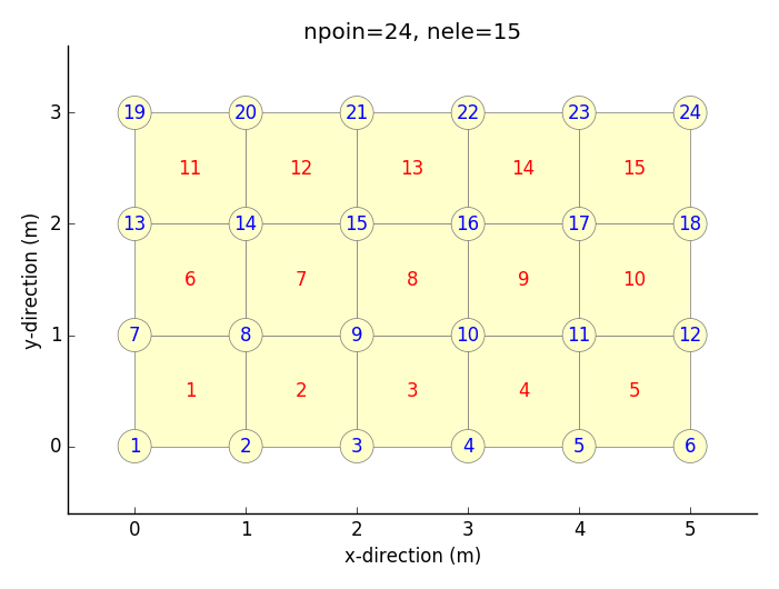
4. Output sample
4.1 Execution command
python py_rectmesh.py 5 3 5 3 0 0 > _test.txt
4.2 Output data
Number of nodes, number of elements, element-node relationship and node coordinats are included in output data.
In the last column of a row of element-node relationship, element numbers are writen as reference data.
And in the last column of a row of node coordinates, node numbers are writen as reference data.
   24    15                 # number of nodes, number of elements
    1    2    8    7    1   # element-node relationship
    2    3    9    8    2   # node-1, node-2, node-3, node-4, element_number(reference)
    3    4   10    9    3
    4    5   11   10    4
    5    6   12   11    5
    7    8   14   13    6
    8    9   15   14    7
    9   10   16   15    8
   10   11   17   16    9
   11   12   18   17   10
   13   14   20   19   11
   14   15   21   20   12
   15   16   22   21   13
   16   17   23   22   14
   17   18   24   23   15
     0.000     0.000    1  # x-coordinate, y-coordinate, node_number(reference)
     1.000     0.000    2
     2.000     0.000    3
     3.000     0.000    4
     4.000     0.000    5
     5.000     0.000    6
     0.000     1.000    7
     1.000     1.000    8
     2.000     1.000    9
     3.000     1.000   10
     4.000     1.000   11
     5.000     1.000   12
     0.000     2.000   13
     1.000     2.000   14
     2.000     2.000   15
     3.000     2.000   16
     4.000     2.000   17
     5.000     2.000   18
     0.000     3.000   19
     1.000     3.000   20
     2.000     3.000   21
     3.000     3.000   22
     4.000     3.000   23
     5.000     3.000   24
4.3 Output drawing
2D Frame Analysis
1. Outline
- This is a program for 2D frame analysis. Elastic and small displacement problems can be treated.
- Beam element with 2 nodes is used. 1 node has 3 degrees of freedom in horizontal displacement, vertical displacement and rotation.
- Nodal external force, nodal forced displacement, nodal temperature change and inertia force for element can be given as loads.
- In coordinate system, x-direction is defined as right-direction, y-direction is defined as upward direction and counterclockwise direction is defined as positive in rotation.
- Simultaneous linear equations are solved using numpy.linalg.solve(A, b).
- Input/Output file name can be defined arbitrarily with the format of space separater and those are inputted as command line arguments of a terminal.
| Valid boundary conditions |
|---|
| Item | Description |
|---|
| External force | Specify the loded nodes and load values |
| Temperature change | Specify the temperature change at all nodes |
| Inertia force | Specify the inertia force as a ratio to the gravity acceleration in horizontal and vertical direction in the material properties data |
| Forced displacement | Specify the nodes with forced displacements and those values. Any values can be applied including zero |
2. FEM program
3. Command format for FEM analysis execution
python3 py_fem_frame.py inp.txt out.txt
| inp.txt | : Input data file (separated by space) |
| out.txt | : Output data file (separated by space) |
4. Input data format
npoin  nele  nsec  npfix  nlod                   # Basic values for analysis
E  A  I  alpha  gamma  gkh  gkv                  # Material properties
    ..... (1 to nsec) .....                      #
node_1  node_2  isec                             # Element connectivity, material set number
    ..... (1 to nele) .....                      #
x  y  deltaT                                     # Node coordinate, temperature change of node
    ..... (1 to npoin) .....                     #
lp  fix_x  fix_y  fix_r  rdis_x  rdis_y  rdis_r  # Restricted node and restrict conditions
    ..... (1 to npfix) .....                     #
lp  fp_x  fp_y  fp_r                             # Loaded node and loading conditions
    ..... (1 to nlod) .....                      #     (omit data input if nlod=0)
| npoin, nele, nsec | : number of nodes, number of elements, number of material sets |
| npfix, nlod | : number of restricted nodes, number of loaded nodes |
| E, A, I, alpha | : elastic modulus, section area, moment of inertia, thermal expansion coefficient |
| gamma, gkh, gkv | : unit weight, horizontal and vertical acceleration (ratio to 'g') |
| node_1, node_2, isec | : node-1, node-2, material set number |
| x, y, deltaT | : x-coordinate, y-coordinate, nodal temperature change |
| lp, fix_x, fix_y, fix_r | : node, kind of restriction in x, y and rotation (0: free, 1: fixed) |
| rdis_x, rdis_y, rdis_r | : forced displacement in x, y and rotation (input zero even if no-restriction) |
| lp, fp_x, fp_y, fp_r | : loaded node, loads in x, y and rotation |
5. Output data format
npoin  nele  nsec npfix  nlod
    (Each value of above)
sec  E  A  I  alpha  gamma  gkh  gkv
    sec   : Material number
    E     : Elastic modulus
    A     : Section area
    I     : Moment of inertia
    alpha : Thermal expansion coefficient
    gamma : Unit weight
    gkh   : Acceleration in horizontal direction (ratio to g)
    gkv   : Acceleration in vertical direction (ratio to g)
    ..... (1 to nsec) .....
node  x  y  fx  fy  fr  deltaT  kox  koy  kor
    node   : Node number
    x      : x-coordinate
    y      : y-coordinate
    fx     : Load in x-direction
    fy     : Load in y-direction
    fr     : Moment load
    deltaT : Temperature change of node
    kox    : Index of restriction in x-direction (0: free, 1: fixed)
    koy    : Index of restriction in y-direction (0: free, 1: fixed)
    kor    : Index of restriction in rotation    (0: free, 1: fixed)
    ..... (1 to npoin) .....
node  kox  koy  kor  rdis_x  rdis_y  rdis_r
    node    : Node number
    kox     : Index of restriction in x-direction (0: free, 1: fixed)
    koy     : Index of restriction in y-direction (0: free, 1: fixed)
    kor     : Index of restriction in rotation    (0: free, 1: fixed)
    rdis_x  : Given displacement in x-direction
    rdis_y  : Given displacement in y-direction
    rdis_r  : Given displacement in rotation
    ..... (1 to npfix) .....
elem  i  j  sec
    elem : Element number
    i    : Node number of start point
    j    : Node number of end point
    sec  : Material number
    ..... (1 to nele) .....
node  dis-x  dis-y  dis-r
    node  : Node number
    dis-x : Displacement in x-direction
    dis-y : Displacement in y-direction
    dis-r : Displacement in rotation
    ..... (1 to npoin) .....
elem  N_i  S_i  M_i  N_j  S_j  M_j
    elem : Element number
    N_i  : Axial force of node-i
    S_i  : Shear force of node-i
    M_i  : Moment of node-i
    N_j  : Axial force of node-j
    S_j  : Shear force of node-j
    M_j  : Moment of node-j
    ..... (1 to nele) .....
n=(total degrees of freedom)  time=(calculation time)
| dis-x, dis-y, dis-r | : displacements in x, y and rotation |
| N, S, M | : axial force, shearing force, moment |
| n | : Total degrees of freedom (the number of the variables) |
| time | : Calculation time |
6. Output sample
6.1 Input data sample and auxiliary program
| Program name | Description |
|---|
| inp_frm.txt | Input data sample for FEM analysis |
| py_fig_force.py | Drawing program of section force diagrams (matplotlib) |
6.2 Outline of sample analysis model
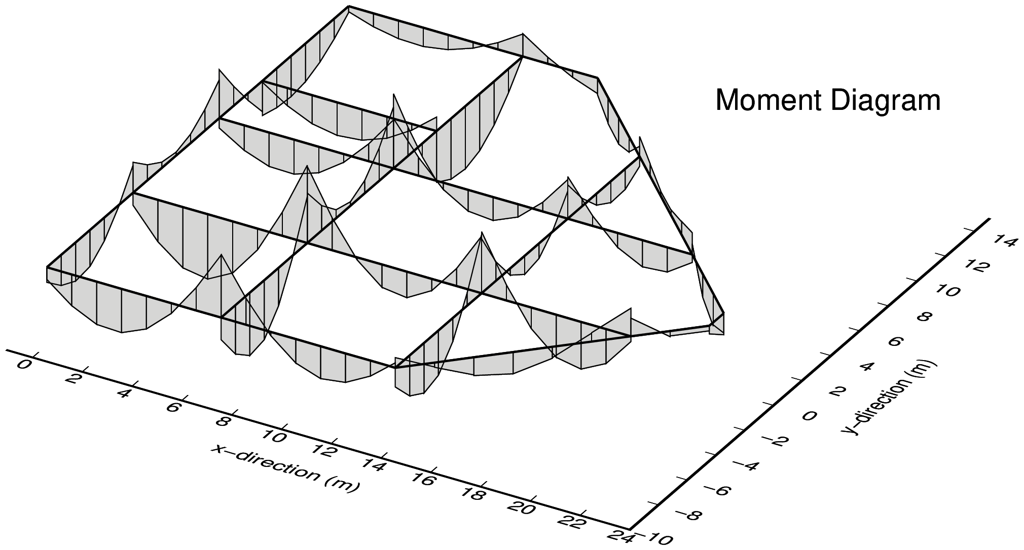
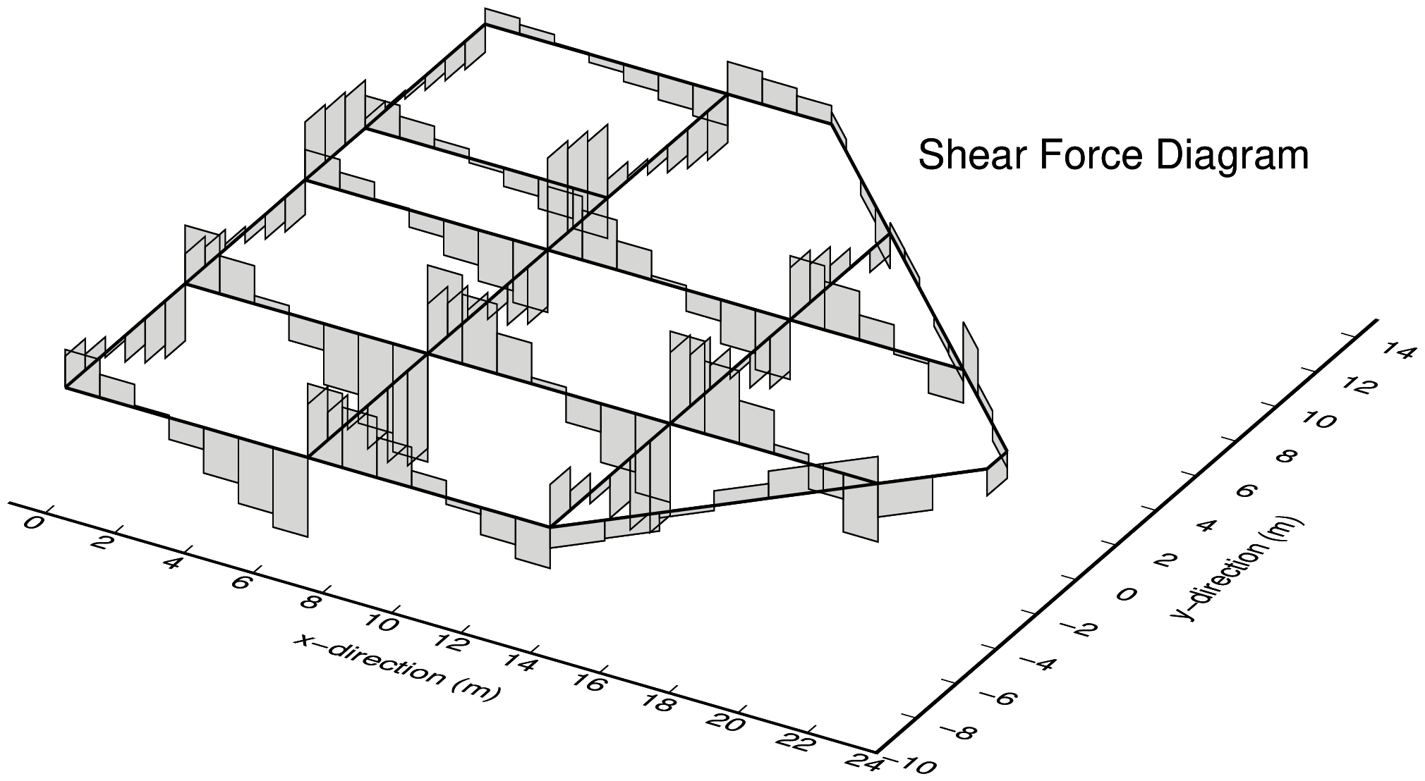
Sample analysis model is a concrete box culvert under the vertical load, lateral soil pressure and uplift. Model is simply supported below the 3 walls.
6.3 Execution command for FEM analysis and drawing
python3 py_fem_frame.py inp_frm.tst out_frm.txt
python3 py_fig_force.py out_frm.txt
| out_frm.txt | : output data file of FEM analysis (saparated by space) |
Section force diagram drawong program creates following image files automatically.
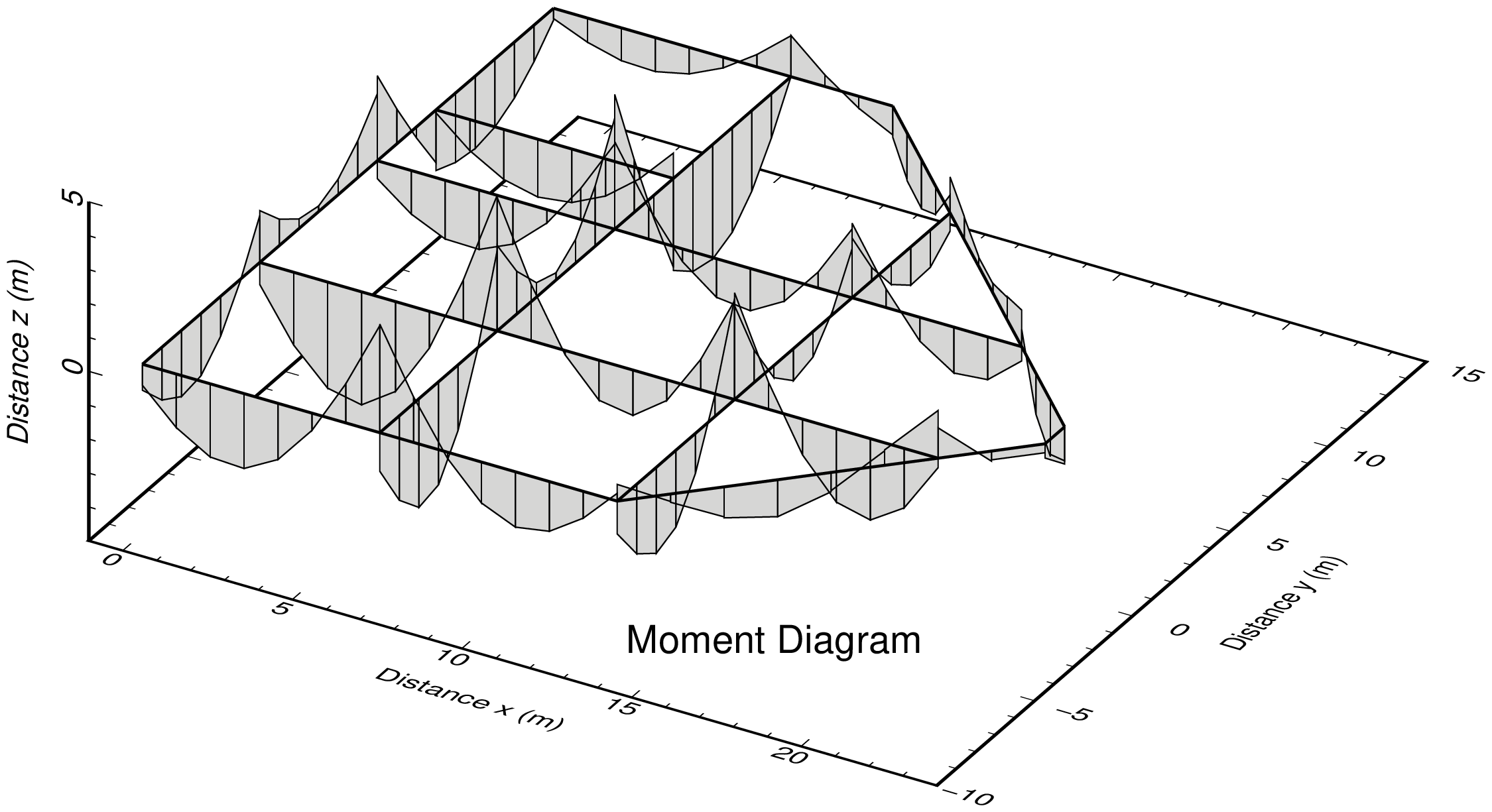
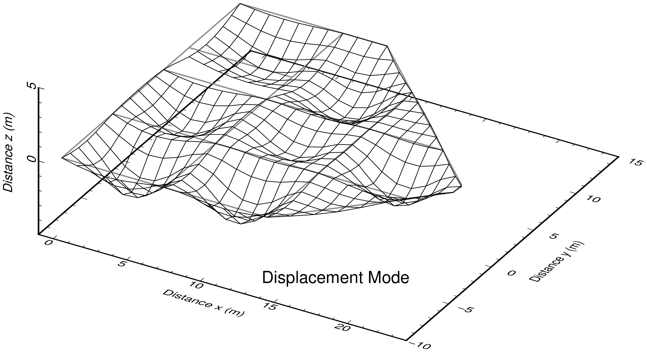
| fig_dis.png | : displacement mode diagram |
| fig_axi.png | : axial force diagram |
| fig_she.png | : shearing force diagram |
| fig_mom.png | : moment diagram |
The commands for specifing drawing range and scale should be re-writed if necessary.
axmin=np.min(x)
axmax=np.max(x)
aymin=np.min(y)
aymax=np.max(y)
midx=0.5*(axmin+axmax)
midy=0.5*(aymin+aymax)

dr=np.min([axmax-axmin,aymax-aymin])
scl_dis=0.2*dr
scl_axi=0.2*dr
scl_she=0.2*dr
scl_mom=0.3*dr
ddmax=np.max([scl_dis,scl_axi,scl_she,scl_mom])
xmin=midx-(midx-axmin+ddmax)*1.1
xmax=midx+(axmax-midx+ddmax)*1.1
ymin=midy-(midy-aymin+ddmax)*1.1
ymax=midy+(aymax-midy+ddmax)*1.6
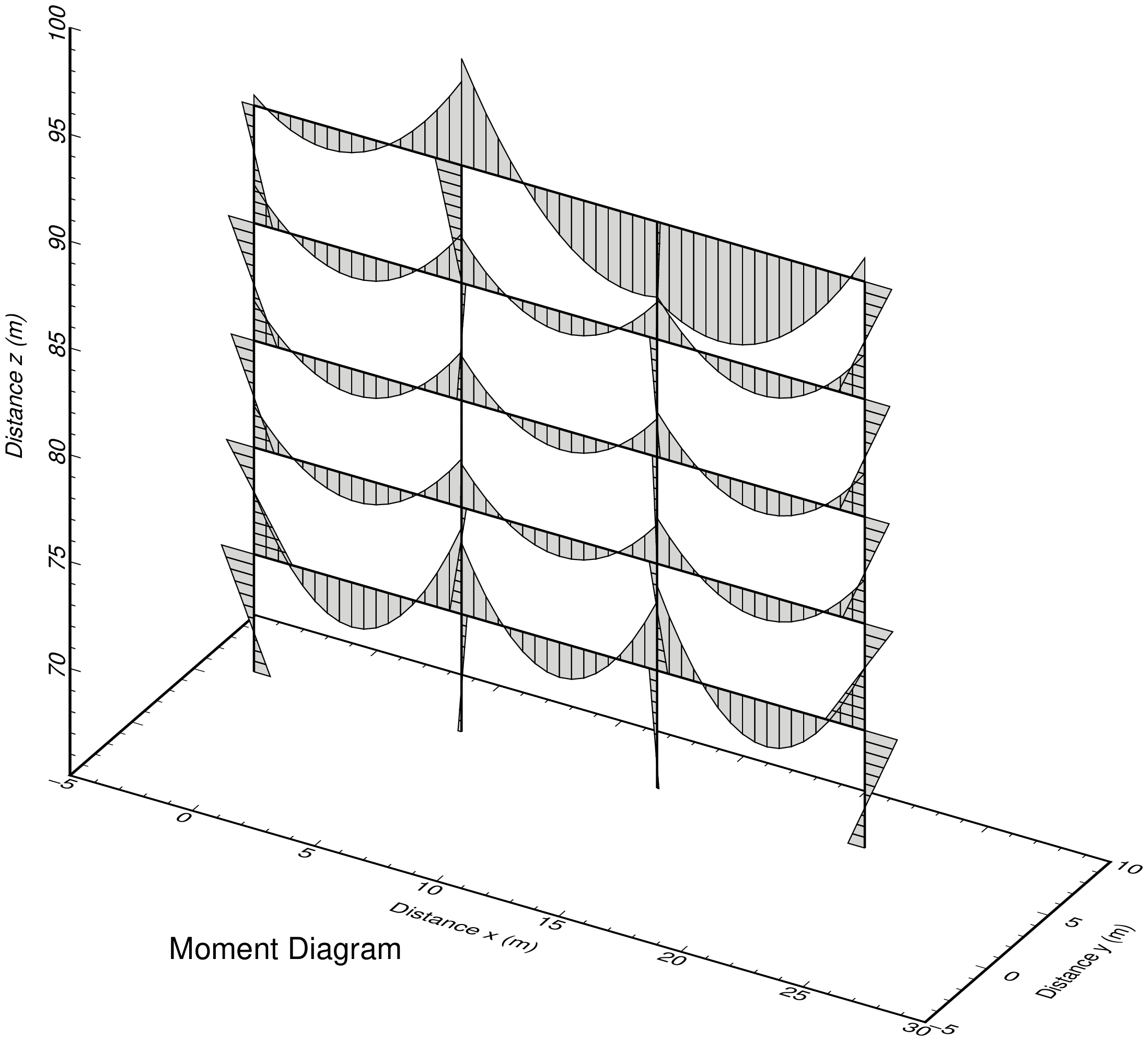
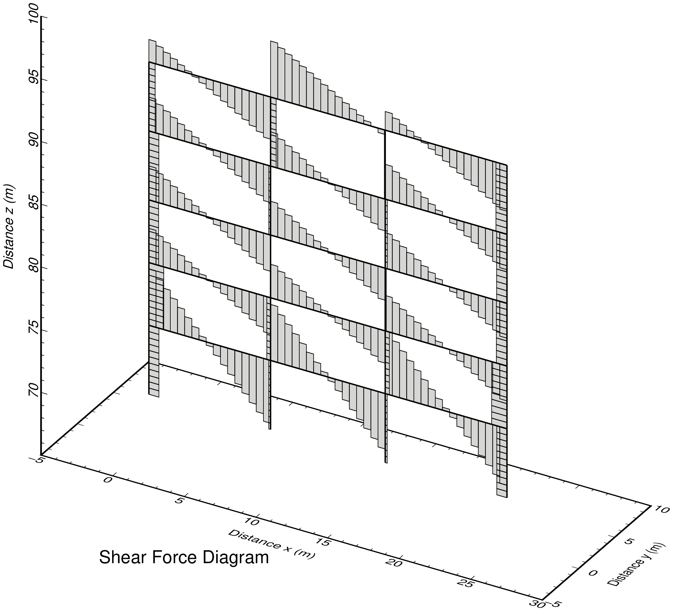
6.4 Sample of section force diagrams
2D Truss Analysis
1. Outline
- This is a program for 2D truss analysis. Elastic and small displacement problems can be treated.
- Truss element with 2 nodes is used. 1 node has 2 degrees of freedom in horizontal displacement and vertical displacement.
- Nodal external force, nodal forced displacement, nodal temperature change and inertia force for element can be given as loads.
- In coordinate system, x-direction is defined as right-direction, y-direction is defined as upward direction.
- Simultaneous linear equations are solved using numpy.linalg.solve(A, b).
- Input/Output file name can be defined arbitrarily with the format of space separater and those are inputted as command line arguments of a terminal.
| Valid boundary conditions |
|---|
| Item | Description |
|---|
| External force | Specify the loded nodes and load values |
| Temperature change | Specify the temperature change at all nodes |
| Inertia force | Specify the inertia force as a ratio to the gravity acceleration in horizontal and vertical direction in the material properties data |
| Forced displacement | Specify the nodes with forced displacements and those values. Any values can be applied including zero |
2. FEM program
3. Command format for FEM analysis execution
python3 py_fem_truss.py inp.txt out.txt
| inp.txt | : Inpyt data file (separated by space) |
| out.txt | : Output data file (separated by space) |
4. Input data format
npoin  nele  nsec  npfix  nlod    # Basic values for analysis
E  A  alpha  gamma  gkh  gkv      # Material properties
    ..... (1 to nsec) .....       #
node_1  node_2  isec              # Element connectivity, material set number
    ..... (1 to nele) .....       #
x  y  deltaT                      # Node coordinate, temperature change of node
    ..... (1 to npoin) .....      #
lp  fix_x  fix_y  rdis_x  rdis_y  # Restricted node and restrict conditions
    ..... (1 to npfix) .....      #
lp  fp_x  fp_y                    # Loaded node and loading conditions
    ..... (1 to nlod) .....       #     (omit data input if nlod=0)
| npoin, nele, nsec | : number of nodes, number of elements, number of material sets |
| npfix, nlod | : number of restricted nodes, number of loaded nodes |
| E, A, alpha | : elastic modulus, section area, thermal expansion coefficient |
| gamma, gkh, gkv | : unit weight, horizontal and vertical acceleration (ratio to 'g') |
| node_1, node_2, isec | : node-1, node-2, material set number |
| x, y, deltaT | : x-coordinate, y-coordinate, nodal temperature change |
| lp, fix_x, fix_y | : node, kind of restriction in x and y direction (0: free, 1: fixed) |
| rdis_x, rdis_y | : forced displacement in x and y direction (input zero even if no-restriction) |
| lp, fp_x, fp_y | : loaded node, loads in x and y direction |
5. Output data format
npoin  nele  nsec npfix  nlod
    (Each value of above)
sec  E  A  alpha  gamma  gkh  gkv
    sec   : Material number
    E     : Elastic modulus
    A     : Section area
    alpha : Thermal expansion coefficient
    gamma : Unit weight
    gkh   : Acceleration in horizontal direction (ratio to g)
    gkv   : Acceleration in vertical direction (ratio to g)
    ..... (1 to nsec) .....
node  x  y  fx  fy  fr  deltaT  kox  koy  kor
    node   : Node number
    x      : x-coordinate
    y      : y-coordinate
    fx     : Load in x-direction
    fy     : Load in y-direction
    deltaT : Temperature change of node
    kox    : Index of restriction in x-direction (0: free, 1: fixed)
    koy    : Index of restriction in y-direction (0: free, 1: fixed)
    ..... (1 to npoin) .....
node  kox  koy  kor  rdis_x  rdis_y  rdis_r
    node    : Node number
    kox     : Index of restriction in x-direction (0: free, 1: fixed)
    koy     : Index of restriction in y-direction (0: free, 1: fixed)
    rdis_x  : Given displacement in x-direction
    rdis_y  : Given displacement in y-direction
    ..... (1 to npfix) .....
elem  i  j  sec
    elem : Element number
    i    : Node number of start point
    j    : Node number of end point
    sec  : Material number
    ..... (1 to nele) .....
node  dis-x  dis-y
    node  : Node number
    dis-x : Displacement in x-direction
    dis-y : Displacement in y-direction
    ..... (1 to npoin) .....
elem  N_i  S_i  N_j  S_j
    elem : Element number
    N_i  : Axial force of node-i
    S_i  : Shear force of node-i
    N_j  : Axial force of node-j
    S_j  : Shear force of node-j
    ..... (1 to nele) .....
n=(total degrees of freedom)  time=(calculation time)
| dis-x, dis-y | : displacements in x and y-direction |
| N, S | : axial force, shearing force |
| n | : Total degrees of freedom (the number of the variables) |
| time | : Calculation time |
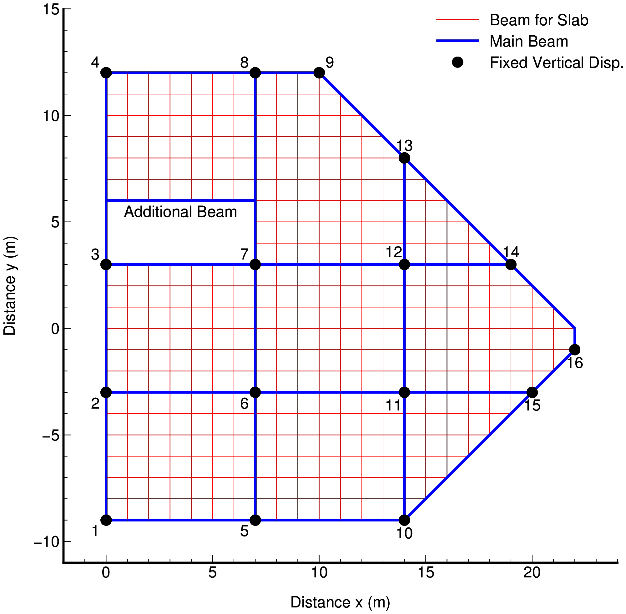
Grid Girder Analysis
1. Outline
- This is a program for grid girder analysis. Elastic and small displacement problems can be treated.
- Beam element with 2 nodes is used. 1 node has 3 degrees of freedom in torsional rotation, bending rotation and vertical displacement.
- Nodal external force and nodal forced displacement can be given as loads.
- A grid girder structure shall be arranged on x-y plane in the global coordinate system.
- Axial direction of a member corresponds to x-axis of local coordinate system.
- The tortional rotation corresponds to the rotation around x-axis in local coordinate system.
- The bending rotation corresponds to the rotation around y-axis in local coordinate system.
- The deflection of grid girder corresponds to the displacement in z-direction in local coordinate system, and this value is the same as the displacement in global coordinate system.
- Simultaneous linear equations are solved using numpy.linalg.solve(A, b).
- Input/Output file name can be defined arbitrarily with the format of space separater and those are inputted as command line arguments of a terminal.
| Valid boundary conditions |
|---|
| Item | Description |
|---|
| External force | Specify the loded nodes and load values |
| Forced displacement | Specify the nodes with forced displacements and those values. Any values can be applied including zero |
2. FEM program
3. Command format for FEM analysis execution
python3 py_fem_grid.py inp.txt out.txt
| inp.txt | : Input data file (separated by space) |
| out.txt | : Output data file (separated by space) |
4. Input data format
npoin  nele  nsec  npfix  nlod                   # Basic values for analysis
E  po  A  I  J                                   # Material properties
    ..... (1 to nsec) .....                      #
node_1  node_2  isec  qw                         # Element connectivity, material set number, load
    ..... (1 to nele) .....                      #
x  y                                             # Node coordinate
    ..... (1 to npoin) .....                     #
lp  fix_x  fix_y  fix_z  rdis_x  rdis_y  rdis_z  # Restricted node and restrict conditions
    ..... (1 to npfix) .....                     #
lp  fp_x  fp_y  fp_z                             # Loaded node and loading conditions
    ..... (1 to nlod) .....                      #     (omit data input if nlod=0)
| npoin, nele, nsec | : number of nodes, number of element, number of material sets |
| npfix, nlod | : number of restricted nodes, number of loaded nodes |
| E, po, A, I, J | : elastic modulus, poisson's ratio, section area, moment of inertia, torsional constant |
| node_1, node_2, isec, qw | : node-1, node-2, material set number |
| x, y | : x-coordinate, y-coordinate |
| lp, fix_x, fix_y, fix_z | : node, kind of restriction in torsion, bending and vertical deflection (0: free, 1: fixed) |
| rdis_x, rdis_y, rdis_z | : forced displacement in tortion, bending and vertical defrection (input zero even if no-restriction) |
| lp, fp_x, fp_y, fp_z | : node, loads in tortional, bending and vertical. |
Although a shear modulus $G$ is required in the grid girder analysis, it is calculated from a elastic modulus ($E$, E) and Poisson's ratio ($\nu$, po) using following relationship in this program.
\begin{equation}
G=\cfrac{E}{2 (1+\nu)}
\end{equation}
5. Output data format
npoin  nele  nsec npfix  nlod
    (Each value of above)
sec  E  po  A  I  J
    sec   : Material number
    E     : Elastic modulus
    po    : Poisson's ratio
    A     : Section area
    I     : Moment of inertia
    J     : Tortional constant
    ..... (1 to nsec) .....
node  x  y  fx  fy  fz  kox  koy  koz
    node   : Node number
    x      : x-coordinate
    y      : y-coordinate
    fx     : Tortional moment load around x-axis
    fy     : Bending moment load
    fz     : Vertical load
    kox    : Index of restriction in tortional rotationin (0: free, 1: fixed)
    koy    : Index of restriction in bending rotation     (0: free, 1: fixed)
    koz    : Index of restriction in vertical direction   (0: free, 1: fixed)
    ..... (1 to npoin) .....
node  kox  koy  kor  rdis_x  rdis_y  rdis_r
    node    : Node number
    kox     : Index of restriction in tortional rotationin (0: free, 1: fixed)
    koy     : Index of restriction in bending rotation     (0: free, 1: fixed)
    koz     : Index of restriction in vertical direction   (0: free, 1: fixed)
    rdis_x  : Given rotation by tortional moment
    rdis_y  : Given rotation by bending moment
    rdis_z  : Given displacement in z (vertical) direction
    ..... (1 to npfix) .....
elem  i  j  sec
    elem : Element number
    i    : Node number of start point
    j    : Node number of end point
    sec  : Material number
    qw   : uniformly distributed vertical load per unit length
    ..... (1 to nele) .....
node  dis-x  dis-y  dis-r
    node  : Node number
    dis-x : Rotation by tortional moment
    dis-y : Rotation by bending moment
    dis-z : Vertical displacement
    ..... (1 to npoin) .....
elem  T_i  M_i  Q_i  T_j  M_j  Q_j
    elem : Element number
    T_i  : Tortional moment of node-i
    M_i  : Bending moment of node-i
    Q_i  : Shear force of node-i
    T_j  : Tortional moment of node-j
    M_j  : Bending moment of node-j
    Q_j  : Shear force of node-j
    ..... (1 to nele) .....
n=(total degrees of freedom)  time=(calculation time)
| dis-x, dis-y, dis-z | : tortional rotation, bending rotation, vertical deflection |
| T, M, Q | : torque, bending moment, shearing force |
| n | : Total degrees of freedom (the number of the variables) |
| time | : Calculation time |
6. Output sample
6.1 Input data sample and auxiliary program
6.2 Outline of sample analysis model
A model which is pentagon shape grid girder system made by RC is subjected to the vertical distributed loads.
6.3 Execution command for FEM analysis and drawing
python3 py_fem_grid.py inp_grid.txt out_grid.txt  # FEM calculation
python3 py_grid_result.py out_grid.txt            # Data making for GMT drawings
bash a_gmt_result.txt                             # GMT script for drawing
(Reference) ImageMagick command for format change from eps to png
mogrify -trim -density 300 -bordercolor "#ffffff" -border 10x10 -format png *.eps
rm *.eps
6.4 Sample drawings
(1) Drawings of analysis model and loading pattern by GMT
Python program 'py_grid_model.py' and shell script including GMT command 'a_gmt_model.txt' were used for these works.
eps images by GMT were converted to png images by ImageMagick.
 |
 |
| Analysis model of grid girder system | Loading pattern (vertical load) |
|---|
(2) Section force diagrams by GMT
Python program 'py_grid_result.py' and shell script including GMT command 'a_gmt_result.txt' were used for these works.
eps images by GMT were converted to png images by ImageMagick.
3D Frame Analysis
1. Outline
- This is a program for 3D frame analysis. Elastic and small displacement problems can be treated.
- Beam element with 2 nodes is used. 1 node has 6 degrees of freedom in X-Y-Z direction displacements and rotations around X-Y-Z axes.
- Nodal external force, nodal forced displacement, nodal temperature change and inertia force for element can be given as loads.
- In the global coordinate system, Z axis is defined as a vertical axis and X and Y axes are defined as a horizontal plane.
- In the local coordinate system, x axis is defined as the member axis direction and y and z axes are defined as principal axes of a section.
- Simultaneous linear equations are solved using numpy.linalg.solve(A, b).
- Input/Output file name can be defined arbitrarily with the format of space separater and those are inputted as command line arguments of a terminal.
| Valid boundary conditions |
|---|
| Item | Description |
|---|
| External force | Specify the loded nodes and load values |
| Temperature change | Specify the temperature change at all nodes |
| Inertia force | Specify the inertia force as a ratio to the gravity acceleration in X, Y and Z directions in the material properties data |
| Forced displacement | Specify the nodes with forced displacements and those values. Any values can be applied including zero |
2. FEM program
3. Command format for FEM analysis execution
python3 py_fem_3dfrm.py inp.txt out.txt
| inp.txt | : Input data file (separated by space) |
| out.txt | : Output data file (separated by space) |
4. Input data format
npoin  nele  nsec  npfix  nlod                   # Basic values for analysis
E  po  A  Ix  Iy  Iz  theta  alpha  gamma  gkX  gkY  gkZ
    ..... (1 to nsec) .....                      # Material properties
node_1  node_2  isec                             # Element connectivity, material set number
    ..... (1 to nele) .....                      #
x  y  z  deltaT                                  # Node coordinate, temperature change of node
    ..... (1 to npoin) .....                     #
lp  kox  koy  koz  kmx  kmy  kmz  rdis_x  rdis_y  rdis_z  rrot_x  rrot_y  rrot_z
    ..... (1 to npfix) .....                     # Restricted node and restrict conditions
lp  fp_x  fp_y  fp_z  mp_x  mp_y  mp_z           # Loaded node and loading conditions
    ..... (1 to nlod) .....                      #     (omit data input if nlod=0)
npoin, nele, nsec       : number of nodes, number of elements, number of material sets
npfix, nlod             : number of restricted nodes, number of loaded nodes
E, po, A                : elastic modulus, Poisson's ratio, section area
Ix, Iy, Iz, theta       : torsional constant, moment of inertia around y-axis or z-axis, chord angle
alpha, gamma            : thermal expansion coefficient, unit weight of material
gkX, gkY, gkZ           : accelerations in X, Y and Z directions (ratio to 'g')
node-1, node-2, isec    : node-1, node-2, material set number
x, y, z, deltaT         : (x,y,z) coordinate of node, nodal temperature change
lp,kox,koy,koz          : node, kind of displacement restriction in X, Y and Z directions (0: free, 1: fixed)
   kmx,kmy,kmz          : kind of rotation restriction around X, Y and Z axis (0: free, 1: fixed)
   rdis_x,rdis_y,rdis_z : forced displacements in X, Y and Z direction (input zero iven if no-restriction)
   rrot_x,rrot_y,rrot_z : forced rotations around X, Y and Z axis (input zero even if no-restriction)
lp, fp_x, fp_y, fp_z    : loaded node, loads in X, Y amd Z direction
    mp_x, mp_y, mp_z    : moments around X, Y and Z axis
5. Output data format
npoin  nele  nsec npfix  nlod
    (Each value of above)
sec  E      po     A    J    Iy    Iz    theta
sec  alpha  gamma  gkX  gkY  gkZ
    sec   : Material number
    E     : Elastic modulus
    po    : Poisson's ratio
    A     : Section area
    J     ; Torsional constant
    Iy    : Moment of inertia around y-axis
    Iz    : Moment of inertia around z-axis
    theta : Chord angle
    alpha : Thermal expansion coefficient
    gamma : Unit weight
    gkX   : Acceleration in X-direction (ratio to g)
    gkY   : Acceleration in Y-direction (ratio to g)
    gkZ   : Acceleration in Z-direction (ratio to g)
    ..... (1 to nsec) .....
node   x   y   z   fx   fy   fz   mx   my   mz  deltaT
    node   : Node number
    x      : x-coordinate
    y      : y-coordinate
    fx     : Load in X-direction
    fy     : Load in Y-direction
    fz     : Load in Z-direction
    mx     : Moment load around X-axis
    my     : Moment load around Y-axis
    mz     : Moment load around Z-axis
    deltaT : Temperature change of node
    ..... (1 to npoin) .....
node   kox   koy   koz   kmx   kmy   kmz   rdis_x   rdis_y   rdis_z   rrot_x   rrot_y   rrot_z
    node    : Node number
    kox     : Index of restriction in X-direction (0: free, 1: fixed)
    koy     : Index of restriction in Y-direction (0: free, 1: fixed)
    koz     : Index of restriction in Z-direction (0: free, 1: fixed)
    kmx     : Index of restriction in rotation around X-axis  (0: free, 1: fixed)
    kmy     : Index of restriction in rotation around Y-axis  (0: free, 1: fixed)
    kmz     : Index of restriction in rotation around Z-axis  (0: free, 1: fixed)
    rdis_x  : Given displacement in X-direction
    rdis_y  : Given displacement in Y-direction
    rdis_z  : Given displacement in Z-direction
    rrot_x  : Given displacement in rotation around X-axis
    rrot_y  : Given displacement in rotation around Y-axis
    rrot_z  : Given displacement in rotation around Z-axis
    ..... (1 to npfix) .....
elem     i     j   sec
    elem : Element number
    i    : Node number of start point
    j    : Node number of end point
    sec  : Material number
    ..... (1 to nele) .....
node   dis-x   dis-y   dis-z   rot-x   rot-y   rot-z
    node  : Node number
    dis-x : Displacement in X-direction
    dis-y : Displacement in Y-direction
    dis-z : Displacement in Z-direction
    rot-x : Rotation around X-axis
    rot-y : Rotation around Y-axis
    rot-z : Rotation around Z-axis
    ..... (1 to npoin) .....
elem nodei   N_i   Sy_i   Sz_i   Mx_i   My_i   Mz_i
elem nodej   N_j   Sy_j   Sz_j   Mx_j   My_j   Mz_j
    elem  : Element number
    nodei : First node nymber
    nodej : Second node number
    N_i   : Axial force of node-i
    Sy_i  : Shear force of node-i in y-direction
    Sz_i  : Shear force of node-i in z-direction
    Mx_i  : Moment of node-i around x-axis (torsional moment)
    My_i  : Moment of node-i around y-axis (bending moment)
    Mz_i  : Moment of node-i around z-axis (bending moment)
    N_j   : Axial force of node-j
    Sy_j  : Shear force of node-j in y-direction
    Sz_j  : Shear force of node-j in z-direction
    Mx_j  : Moment of node-j around x-axis (torsional moment)
    My_j  : Moment of node-j around y-axis (bending moment)
    Mz_j  : Moment of node-j around z-axis (bending moment)
    ..... (1 to nele) .....
n=(total degrees of freedom)  time=(calculation time)
6. Output samples
6.1 Control script
python3 py_fem_3dfrm.py inp_3dfrm_grid.txt out_3dfrm_grid.txt
python3 py_fig_3dfrm_grid.py
source a_3dfrm_grid.txt

python3 py_fem_3dfrm.py inp_3dfrm_b3_yz.txt out_3dfrm_b3_yz.txt
python3 py_fig_3dfrm_cpost1.py
source a_3dfrm_cpost1.txt

python3 py_fem_3dfrm.py inp_3dfrm_b3_xz.txt out_3dfrm_b3_xz.txt
python3 py_fig_3dfrm_cpost2.py
source a_3dfrm_cpost2.txt

rm _*
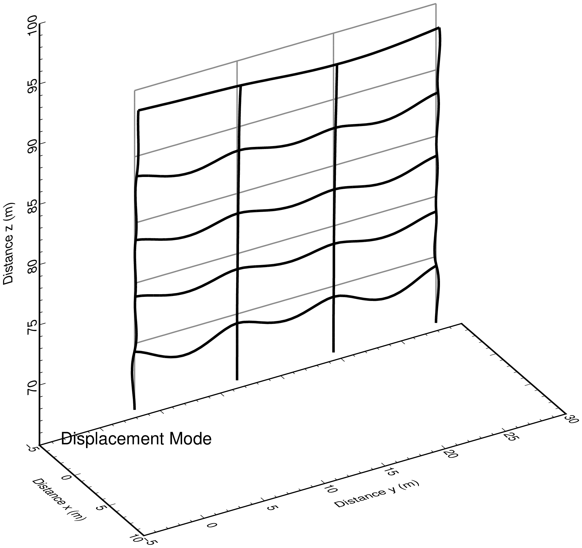
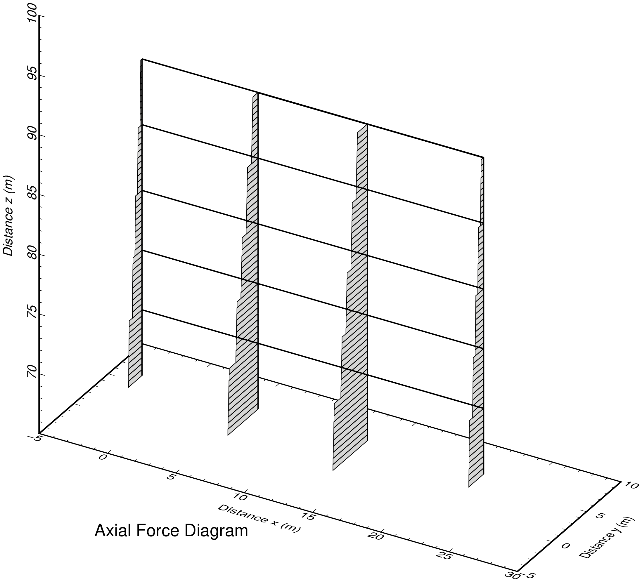
6.2 Input data samples and auxiliary programs
Samples of section force diagrams
Input data file:inp_3dfrm_grid.txt
Input data file:inp_3dfrm_b3_yz.txt
Input data file:inp_3dfrm_b3_xz.txt
2D Stress Analysis
1. Outline
- This is a program for 2D stress analysis including plane strain and plane stress state problem based on elastic and small displacement theorem with isotropic material.
- 4 node isoparametric element with 4 Gauss points is used as a 4 node element. 1 node has 2 degrees of freedom in horizontal direction and vertical direction.
- Nodal external force, nodal forced displacement, nodal temperature change and inertia force for element can be given as loads.
- In coordinate system, x-direction is defined as right-direction, y-direction is defined as upward direction.
- Simultaneous linear equations are solved using numpy.linalg.solve(A, b).
- Input/Output file name can be defined arbitrarily with the format of space separater and those are inputted as command line arguments of a terminal.
| Valid boundary conditions |
|---|
| Item | Description |
|---|
| External force | Specify the loded nodes and load values |
| Temperature change | Specify the temperature change at all nodes |
| Inertia force | Specify the inertia force as a ratio to the gravity acceleration in horizontal and vertical direction in the material properties data |
| Forced displacement | Specify the nodes with forced displacements and those values. Any values can be applied including zero |
2. FEM program
3. Command format for FEM analysis execution
python3 py_fem_pl4.py inp.txt out.txt
| inp.txt | : Input data file (separated by space) |
| out.txt | : Output data file (separated by space) |
4. Input data format
npoin  nele  nsec  npfix  nlod  NSTR  # Basic values for analysis
t  E  po  alpha  gamma  gkh  gkv      # Material properties
    ..... (1 to nsec) .....           #
node1  node2  node3  node4  isec      # Element connectivity, material set number
    ..... (1 to nele) .....           #   (counter-clockwise order of node number)
x  y  deltaT                          # Coordinate, Temperature change of node
    ..... (1 to npoin) .....          #
node  kox  koy  rdisx  rdisy          # Restricted node and restrict conditions
    ..... (1 to npfix) .....          #
node  fx  fy                          # Loaded node and loading conditions
    ..... (1 to nlod) .....           #   (omit data input if nlod=0)
| npoin, nele, nsec | : number of nodes, number of elements, number of material sets |
| npfix, nlod | : number of restricted nodes, number of loaded nodes |
| NSTR | : Stress state (0: plane strain, 1: plane stress) |
| t, E, po, alpha | : element thickness, elastic modulus, Poisson's ratio, thermal expansion coefficient |
| gamma, gkh, gkv | : unot weight, horizontal and vertical acceleration (ratio to 'g') |
| node1, node2, node3, node4, isec | : node1, node2, node3, node4, material set number |
| x, y, deltaT | : x-coordinate, y-coordinate, nodal temperature change |
| node, kox, koy | : node, kind of restriction in x and y direction (0: free, 1: fixed) |
| rdisx, rdisy | : forced displacements in x and y-directions (input zero even if no-restriction) |
| node, fx, fy | : loaded node, load in x and y-direction |
5. Output data format
npoin  nele  nsec npfix  nlod   NSTR
    (Each value of above)
sec  t  E  po  alpha  gamma  gkh  gkv
    sec   : Material number
    t     : Element thickness
    E     : Elastic modulus
    po    : Poisson's ratio
    alpha : Thermal expansion coefficient
    gamma : Unit weight
    gkh   : Acceleration in x-direction (ratio to g)
    gkv   : Acceleration in y-direction (ratio to g)
    ..... (1 to nsec) .....
node  x  y  fx  fy  deltaT  kox  koy
    node   : Node number
    x      : x-coordinate
    y      : y-coordinate
    fx     : Load in x-direction
    fy     : Load in y-direction
    deltaT : Temperature change of node
    kox    : Index of restriction in x-direction (0: free, 1: fixed)
    koy    : Index of restriction in x-direction (0: free, 1: fixed)
    ..... (1 to npoin) .....
node  kox  koy  rdis_x  rdis_y
    node    : Node number
    kox     : Index of restriction in x-direction (0: free, 1: fixed)
    koy     : Index of restriction in y-direction (0: free, 1: fixed)
    rdis_x  : Given displacement in x-direction
    tdis_y  : Given displacement in y-direction
    ..... (1 to npfix) .....
elem  i  j  k  l  sec
    elem : Element number
    i    : Node number of start point
    j    : Node number of second point
    k    : Node number of third point
    l    : Node number of end point
    sec  : Material number
    ..... (1 to nele) .....
node  dis-x  dis-y
    node  : Node number
    dis-x : Displacement in x-direction
    dis-y : Displacement in y-direction
    ..... (1 to npoin) .....
elem  sig_x  sig_y  tau_xy  p1  p2  ang
    elem   : Element number
    sig_x  : Normal stress in x-direction
    sig_y  : Normal stress in y-direction
    tau_xy : Shear stress in x-y plane
    p1     : First principal stress
    p2     : Second principal stress
    ang    : Angle of the first principal stress
    ..... (1 to nele) .....
n=(total degrees of freedom)  time=(calculation time)
| dis-x, dis-y | : displacements in x and y-directions |
| sig_x, sig_y, tau_xy | : normal stresses in x and y-direction, shearing stress |
| p1, p2, ang | : !st principal stress, 2nd principal stress, angle of 1st principal stress |
| n | : Total degrees of freedom (the number of the variables) |
| time | : Calculation time |
6. Output sample
6.1 Input data sample and auxiliary program
6.2 Outline of sample analysis model
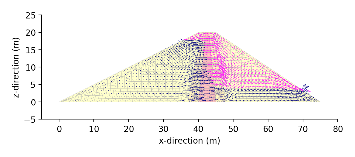
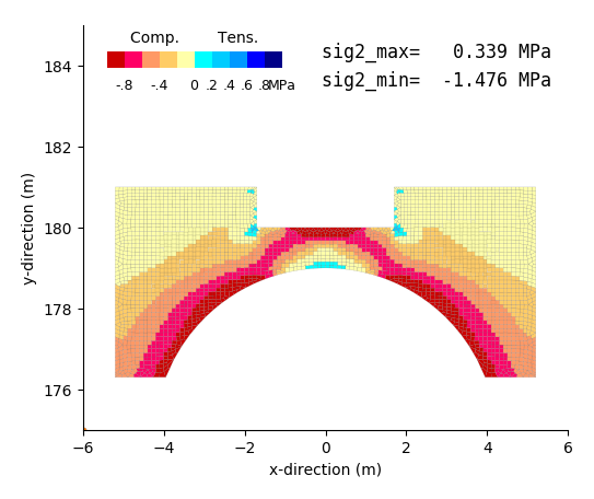
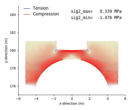
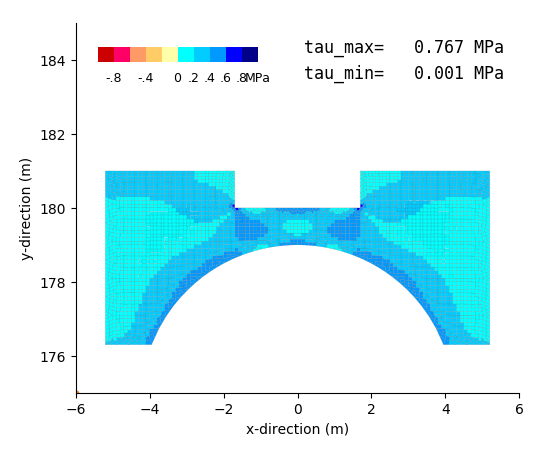
Model is an RC arch with wide notch at center of the arch. The loads subjected are vertical distributed load on wide notch and self weight of the concrete.
6.3 Execution command for FEM analysis and drawing
python3 py_fem_pl4.py inp_arch.txt out_arch.txt
python3 py_fig_cont_pl4.py out_arch.txt
python3 py_fig_vect_pl4.py out_arch.txt
| out_arch.txt | : output data file by FEM analysis (separated by space) |
The drawing programs create following images automatically.
py_fig_cont.py
| _fig_pl4_con1.png | : 1st principal stress color contour |
| _fig_pl4_con2.png | : 2nd principal stress color contour |
| _fig_pl4_con3.png | : maximum shearing stress color contour |
py_fig_vect.py
| _fig_pl4_disp.png | : displacement mode diagram |
| _fig_pl4_vec1.png | : 1st principal stress vector diagram |
| _fig_pl4_vec2.png | : 2nd principal stress vector diagram |
In these programs, drawing range, clasification of stress value and its color, drawing scales of displacement and stress values shall be rewriten properly considering the analysis results.
6.4 Sample drawings
png image drawings which were established by programs 'py_fig_cont_pl4.py' and 'py_fig_vect_pl4.py' are shown below.
 |
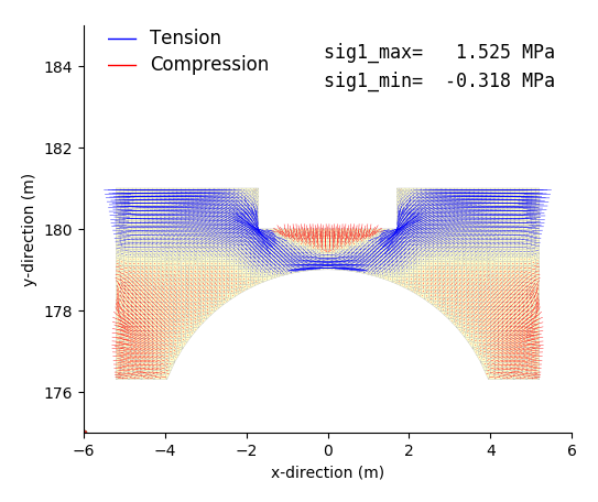 |
| First principal stress contour | First principal stress vector |
|---|
 |
 |
| Second principal stress contour | Second principal stress vector |
|---|
 |
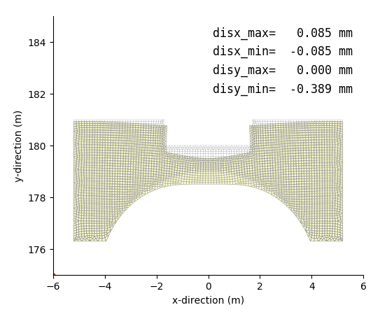 |
| Maximum shearing stress contour | Disolacement mode |
|---|
Axisymmetric Stress Analysis
1. Outline
- This is a program for qxisymmetric stress analysis based on elastic and small displacement theorem with isotropic material.
- 4 node isoparametric element with 4 Gauss points is used as a 4 node element. 1 node has 2 degrees of freedom in rotation axial direction and radial direction.
- Thickness of circumference direction of 1 element is 1 radian.
- Nodal external force, nodal forced displacement, nodal temperature change and inertia force for element in only rotation axis direction can be given as loads.
- In coordinate system, z-direction is defined as rotation axis direction, r-direction is defined as radial direction.
- Simultaneous linear equations are solved using numpy.linalg.solve(A, b).
- Input/Output file name can be defined arbitrarily with the format of space separater and those are inputted as command line arguments of a terminal.
| Valid boundary conditions |
|---|
| Item | Description |
|---|
| External force | Specify the loded nodes and load values |
| Temperature change | Specify the temperature change at all nodes |
| Inertia force | Specify the inertia force as a ratio to the gravity acceleration in horizontal and vertical direction in the material properties data |
| Forced displacement | Specify the nodes with forced displacements and those values. Any values can be applied including zero |
2. FEM program
3. Command format for FEM analysis execution
python3 py_fem_asnt.py inp.txt out.txt
| inp.txt | : Input data file (separated by space) |
| out.txt | : Output file name (separated by space) |
4. Input data format
npoin  nele  nsec  npfix  nlod    # Basic values for analysis
E  po  alpha  gamma  gkz          # Material properties
    ..... (1 to nsec) .....       #
node1  node2  node3  node4  isec  # Element connectivity, material set number
    ..... (1 to nele) .....       #   (counter-clockwise order of node number)
z  r  deltaT                      # Coorinate, temperature change of node
    ..... (1 to npoin) .....      #
node  koz  kor  rdisz  rdisr      # Restricted node and restrict conditions
    ..... (1 to npfix) .....      #   (omit data input if npfix=0)
node  fz  fr                      # Loaded node and loading conditions
    ..... (1 to nlod) .....       #   (omit data input if nlod=0)
| npoin, nele, nsec | : number of nodes, number of elements, number of material sets |
| npfix, nlod | : number of restricted nodes, number of loaded nodes |
| E, po, alpha | : elastic modulus, Poisson's ratio, thermal expansion coefficient |
| gamma, gkz | : unot weight, acceleration in rotation axis direction (ratio to 'g') |
| node1, node2, node3, node4, isec | : node1, node2, node3, node4, material set number |
| z, r, deltaT | : z-coordinate, r-coordinate, nodal temperature change |
| node, koz, kor | : node, kind of restriction in z and r direction (0: free, 1: fixed) |
| rdisz, rdisr | : forced displacements in z and r-directions (input zero even if no-restriction) |
| node, fz, fr | : loaded node, load in z and r-direction |
Explanation of load input method
A cylinder under the internal pressure is considered. The cylinder has the radius of r=3000mm, the length in rotation axial direction of z=200mm and internal pressure of p=1 N/mm2 is acted. Total load acted to 1 element with thickness of 1 radian is shown below.
\begin{align}
&p \times r \times 1 (rad) \times z \\
&= 1 (n/mm^2) \times 3,000 (mm) \times 1 (rad) \times 200 (mm) \\
&= 600,000 (N)
\end{align}
So, below loads must be acted for each node according to the thinking of equivalent nodal force,
| Item | Details |
|---|
| Nodal force | 300,000(N) | 300,000(N) |
| Coordinate of node | (z,r)=(0,3,000) | (z,r)=(200,3,000) |
| Direction of load | Positive radius direction | Positive radius direction |
5. Output data format
npoin  nele  nsec npfix  nlod
    (Each value of above)
sec  E  po  alpha  gamma  gkz
    sec   : Material number
    E     : Elastic modulus
    po    : Poisson's ratio
    alpha : Thermal expansion coefficient
    gamma : Unit weight
    gkz   : Acceleration in rotation axis direction (ratio to g)
    ..... (1 to nsec) .....
node  z  r  fz  fr  deltaT  koz  kor
    node   : Node number
    z      : z-coordinate (rotation axis direction)
    r      : r-coordimate (radial direction)
    fz     : Load in z-direction
    fr     : Load in r-direction
    deltaT : Temperature change of node
    koz    : Index of restriction in z-direction (0: free, 1: fixed)
    kor    : Index of restriction in r-direction (0: free, 1: fixed)
    ..... (1 to npoin) .....
node  koz  kor  rdis_z  rdis_r
    node   :
    koz    : Index of restriction in z-direction (0: free, 1: fixed)
    kor    : Index of restriction in r-direction (0: free, 1: fixed)
    rdis_z : Given displacement in z-direction
    rdis_r : Given displacement in r-direction
    ..... (1 to npfix) .....
elem  i  j  k  l  sec
    elem : Element number
    i    : Node number of start point
    j    : Node number of second point
    k    : Node number of third point
    l    : Node number of end point
    sec  : Material number
    ..... (1 to nele) .....
node  dis-z  dis-r
    node  : Node number
    dis-z : Displacement in z-direction
    dis-r : Displacement in r-direction
    ..... (1 to npoin) .....
elem  sig_z  sig_r  sig_t  tau_zr  p1  p2  ang
    elem   : Element number
    sig_z  : Normal stress in z-direction
    sig_r  : Normal stress in r-direction
    sig_t  : Normal stress in rotation (Third principal stress)
    tau_zr : Shear stress in z-r plane
    p1     : First principal stress in z-r plane
    p2     : Second principal stress in z-r plane
    ang    : Angle of the first principal stress in z-r plane
    ..... (1 to nele) .....
n=(total degrees of freedom)  time=(calculation time)
| dis-z, dis-r | : displacements in z and r directions |
| sig_z, sig_r | : normal stress in z and r directions |
| sig_t | : normal stress in circumference direction to rotation axis (3rd principal stress) |
| p1, p2, ang | : 1st and 2nd principal stresses in z-r plane, angle of 1st principal stress |
| n | : Total degrees of freedom (the number of the variables) |
| time | : Calculation time |
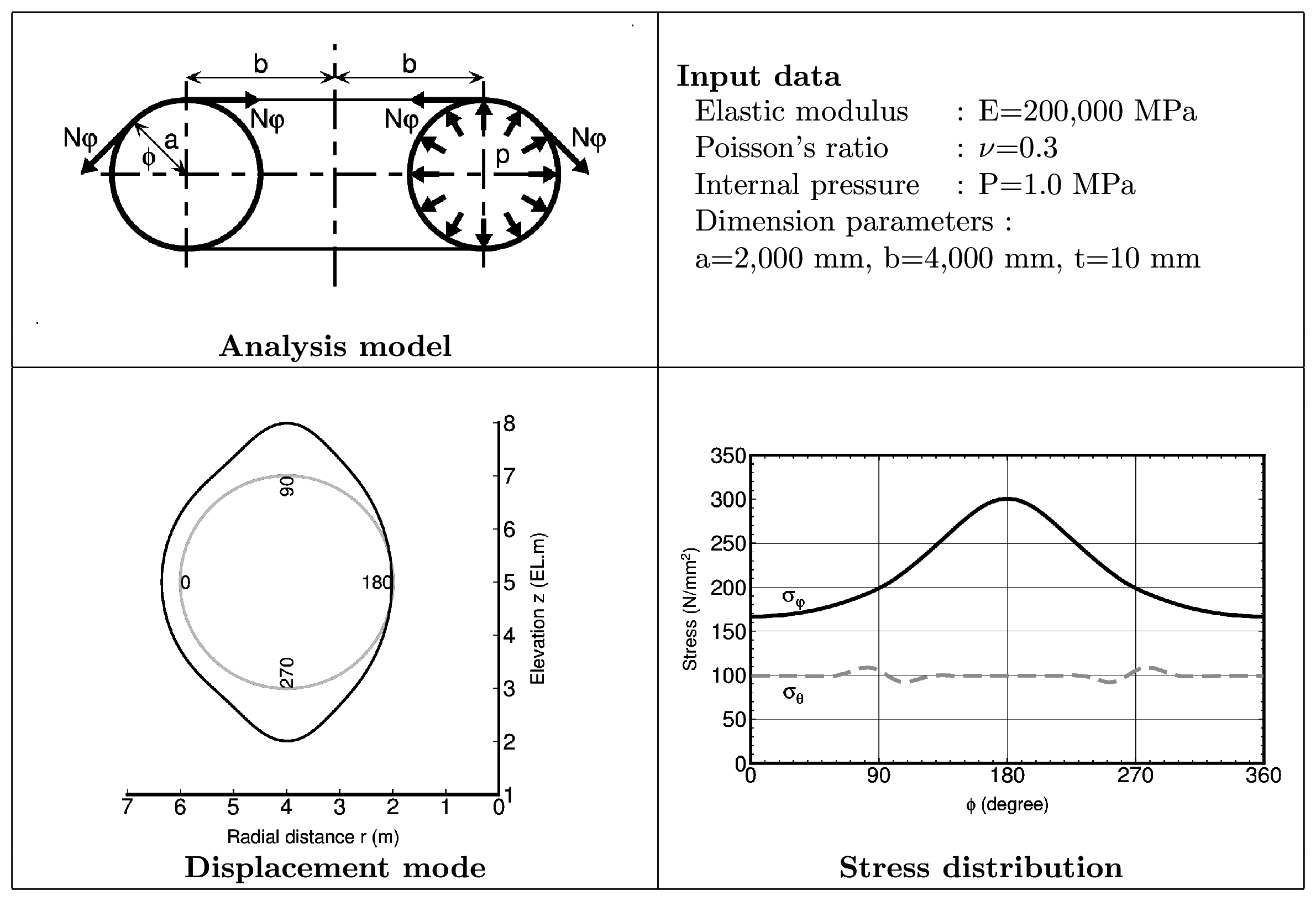
6. Output sample (stress analysis of torus under internal water pressure)
6.1 Input data sample and auxiliary program
6.2 Execution command for FEM analysis and drawing
python3 py_fem_asnt.py inp_torus.txt out_torus.txt
python3 py_fig_data.py out_torus.txt
bash a_gmt_gra.txt
| inp_torus.txt | : Input data file for FEM analysis (separated by space) |
| out_torus.txt | : Output data file by FEM analysis (separated by space) |
6.3 Theoritical solution of stress in torus
A torus shown below left drawing is explained in Wikipedia as following:
A torus is a surface of revolution generated by revolving a circle in three-dimensional space about an axis coplanar with the circle. If the axis of revolution does not touch the circle, the surface has a ring shape and is called a torus of revolution.
When a torus under the uniform internal water pressure is considered shown in above right drawing, the axial force $N_{\varphi}$ in circumferential direction of a circle with radius '$a$' and another axial force $N_{\theta}$ which is perpendicular to previus one are given in following equations which are described in 'Theory of Plates and Shells' by Timoshenko.
\begin{equation}
N_{\varphi}=\cfrac{p a (r_0 + b)}{2 r_0} \qquad\qquad N_{\theta}=\cfrac{p a}{2}
\end{equation}
From above, it can be understood that the value $N_{\varphi}$ is variable depending on the location although the value of $N_{\theta}$ is constant on the circle.
When the values of $N_{\varphi}$ are calculated at some representative points, folowings can be obtained.
\begin{align}
&N_{\varphi}=p a \left\{1 + \cfrac{a}{2(b - a)}\right\} & (r_0 = b - a) \\
&N_{\varphi}=p a & (r_0 = b) \\
&N_{\varphi}=p a \left\{1 - \cfrac{a}{2(b + a)}\right\} & (r_0 = b + a)
\end{align}
From above, the maximum force can be occurred at inside of circle ($r_0 = b - a$).
6.4 FEM Analysis
The results of an axisymmetric stress analysis using a program 'py_fem_asnt.py' are shown below.
Conditions of analysis
Elastic modulus
E (MPa) | Poisson's ratio
po | Internal pressure
p (MPa) | Radius
a (mm) | Radius
b (mm) | Material thickness
t (mm) |
|---|
| 200,000 | 0.3 | 1.0 | 2,000 | 4,000 | 10 |
| number of elements: 360 (center angle: 1 degree) |
The comparison of FEM analyis result and theoritical solution by Timoshenko is shown below.
| Location | FEM | Timoshenko |
|---|
| (φ) | σφ | σθ | σφ | σθ |
|---|
| 0 (r=b+a) | 166.59 | 99.54 | 166.66 | 100.00 |
| 90 (r=b) | 198.43 | 105.62 | 200.00 | 100.00 |
| 180 (r=b-a) | 300.54 | 99.55 | 300.00 | 100.00 |
| unit of stress: MPa |
2D Saturated-Unsaturated Seepage Flow Analysis
1. Outline
- This is a program for 2D steady seepage flow Analysis with isotripic material which is subjected to Darcy's law. This program can not treat unsteady or anisotropic material problem.
- This program can do the saturated-unsaturated seepage flow analysis in the vertical section, and saturated seepage flow analysis in the horizontal and vertical section.
- Von Genuchten model is used as unsaturated ground model.
- 4 node isoparametric element with 4 Gauss points is used as a 4 node element. 1 node has 1 degree of freedom which is nodal total head or nodal discharge
- Thickness of the element is unit thickness and it is not changeable.
- As boundary conditions, impervious boundary, given total head boundary, given discharge boundary and seepage face boundary can be considered.
- In coordinate system, x-direction is defined as right direction and z-direction is defined as upward direction or altitude.
- Nodal head must be inputted as total head and solution of simultaneous equations is described as total head.
- Pressure head is calculated as the difference between total head and position head.
- Simultaneous linear equations are solved using numpy.linalg.solve(A, b).
- Convergence criterion is that the case change of pressure head becomes less than 1$\times$10$^{-6}$.
Upper limit of iteration is set to 100 times.
- Input/Output file name can be defined arbitrarily with the format of space separator and those are inputted from command line of a terminal.
| Valid boundary conditions |
|---|
| Item | Description |
|---|
| Impervious boundary | No-input means impervious boundary |
| Total head given boundary | Specify the nodes and total head |
| Discharge given boundary | Specify the nodes and discharge.
Positive value of discharge means in-flow, and negative value of discharge means out-flow from a element. |
| Seepage face boundary | Specify the nodes which have the possibility of occurance of free surface. Pressure heads at these points are zero or negative value and signs of discharge shall be negative (out-flow) |
Suplimental explanation anout analysis section
- Section for analysis shall be choosen, either vertical or horizontal section.
- In the vartical section calculation, pressure head is given as the difference between total head and position head.
- In the horizontal section analysis, pressure head is the same as total head.
2. FEM program
| Program name | Description |
|---|
| py_fem_seep4.py | 2D Saturated-Unsaturated Seepage Flow Analysis program |
3. Command format for FEM analysis execution
python3 py_fem_seep4.py inp.txt out.txt
| inp.txt | : Input data file (saparated by space) |
| out.txt | : Output data file (separated by space) |
4. Input data format
npoin  nele  nsec  koh  koq  kou  idan  # Basic values for analysis
Ak0  alpha  em                          # Material properties
    ..... (1 to nsec) .....             #
node-1  node-2  node-3  node-4  isec    # Element connectivity
    ..... (1 to nele) .....             #   (counter-clockwise order of node number)
x  z  hvec0                             # Coordinate, initial value of total head
    ..... (1 to npoin) .....            #
nokh  Hinp                              # Node with given total head, given total head
    ..... (1 to koh) .....              #     (omit data input if koh=0)
nokq  Qinp                              # Node with given duscharge, given discharge
    ..... (1 to koq) .....              #     (omit data input if koq=0)
noku                                    # Node with assumed seepage face condition
    ..... (1 to kou) .....              #     (omit data input if kou=0)
| npoin, nele, nsec | : number of nodes, number of elements, number of material sets |
| koh, koq, kou | : number of nodes with given total head, number of nodes with given discharge, number of nodes with assumed seepage face condition |
| idan | : Analysis section (0: vertical, 1: horizontal) |
| Ak0 | : saturated permeability coefficient of element |
| alpa, em | : unsaturated properties of element |
| node-1, node-2, node-3, node-4, isec | : nodes constituting an element, material set number |
| x, z, hvec0 | : x and z coordinate, initial total head for iterative calculation |
| nokh, Hinp | : node with given total head, value of total head |
| nokq, Qinp | : node with given discharge, value of discharge |
| noku | : node with assumed seepage face condition |
5. Output data format
npoin  nele  nsec   koh   koq   kou  idan
    (Each value of above)
sec  Ak0  alpha  em
    Ak0   : Permeability coefficient (saturated)
    alpha : Un-saturated parameter
    em    : Un-saturated parameter
    ..... (1 to nsec) .....
node  x  z  hvec  qvec  koh  koq  kou
    node : Node number
    x    : x-coordinate
    z    : z-coordinate
    hvec : Initial total head
    qvec : Initial discharge
    koh  : Index of node with given total head (0: free, 1: fixed)
    koq  : Index of node with given discharge  (0: free, 1: fixed)
    kou  : Index of node with assumed seepage face (0: free, 1: fixed)
    ..... (1 to npoin) .....
node Hinp
    node : Node number
    Hinp : Given total head
    ..... (1 to koh) .....
node  Qinp
    node : Node number
    Qinp : Given discharge
    ..... (1 to koq) .....
elem  i  j  k  l  sec
    elem : Element number
    i    : Node number of start point
    j    : Node number of second point
    k    : Node number of third point
    l    : Node number of end point
    sec  : Material number
    ..... (1 to nele) .....
node  hvec  pvec  qvec  koh  koq  kou
    node : Node number
    hvec : Total head
    pvec : Pressure head (Total head minus elevation of the node)
    qvec : Discharge (+: inflow, -: outflow)
    koh  : Index of node with given total head (0: free, 1: fixed)
    koq  : Index of node with given discharge  (0: free, 1: fixed)
    kou  : Index of node with assumed seepage face (0: free, 1: fixed)
    ..... (1 to npoin) .....
elem  vx  vz  vm  kr
    elem : Element number
    vx   : Flow velocity in x-direction
    vz   : Flow velocity in z-direction
    vm   : Composed flow velocity
    kr   : Parameter of saturation (1: saturated, less than 1: unsaturated)
    ..... (1 to nele) .....
Total inflow = (total inflow discharge: positive sign)
Total outflow= (total outflow discharge: negative sign)
Max.velocity in all area     =  (maximum velocity in all area)
Max.velocity in inflow area  =  (maximum velocity in inflow area)
Max.velocity in outflow area =  (maximum velocity in outflow area)
iii=(number of itaration)
icount=(converged number of degrees of freedom)
kop=(number of pressured nodes)
n=(total degrees of freedom)  time=(calculation time)
| hvec, pvec, qvec | : total head, pressure head, nodal discharge |
| vx, vz, vm | : velocity in x-direction, velocity in z-direction, composed velocity |
| kr | : Relative hydraulic conductivity function (1: saturated, <1: unsaturated) |
6. Output sample
6.1 Input data sample and auxiliary program
Plotting method of the pressure head contour
Each node coordinate which forms a triangle is set as $(x, z)$, and the value of pressure head is set as $y$.
Under above setting, an equation of a plane passing through 3 points $(x_1,y_1,z_1)$, $(x_2,y_2,z_2)$, $(x_3,y_3,z_3)$ in a 3D space can be defined as follow:
\begin{equation}
a*x+b*y+c*z+d=0
\end{equation}
\begin{align}
a=&(y_2-y_1)*(z_3-z_1)-(y_3-y_1)*(z_2-z_1) \\
b=&(z_2-z_1)*(x_3-x_1)-(z_3-z_1)*(x_2-x_1) \\
c=&(x_2-x_1)*(y_3-y_1)-(x_3-x_1)*(y_2-y_1) \\
d=&-x_1*\{(y_2-y_1)*(z_3-z_1)-(y_3-y_1)*(z_2-z_1)\} \\
&-y_1*\{(z_2-z_1)*(x_3-x_1)-(z_3-z_1)*(x_2-x_1)\} \\
&-z_1*\{(x_2-x_1)*(y_3-y_1)-(x_3-x_1)*(y_2-y_1)\}
\end{align}
And an equation of a line passing through a point $y=y_c$ can be defined as follow:
\begin{align}
z=&-a/c*x-b/c*y_c-d/c \\
=&a'*x+b' \\
&a'=-a/c \\
&b'=-b/c*y_c-d/c
\end{align}
A point $(x_x,z_z)$ which has the minimum distance from a point $(x_g,z_g)$ to a line $z=a'*x+b'$ can be obtained as follow:
\begin{equation}
\begin{cases}
&x_x=\cfrac{x_g+z_g*a'-a'*b'}{1+a'*a'} \\
&z_z=a'*x_x+b'
\end{cases}
\end{equation}
Using above, a point coordinate $(x_x, z_z)$ which has a pressure head value $y_c$ can be calculated.
|
|
It is impossible to create a plane with arbitrary 4 points in the 3D space. Therefore, for 4 nodes elements, the area of element is divided to 4 traiangle areas to create a plane for each triangle area. When the node numbers which forms 4 node element is assumed (1,2,3,4) referring the left drawing, the usable combinations of nodes becomes (1,2,3), (2,3,4), (3,4,1), (4,1,2) with the sequence of counterclockwise direction.
|
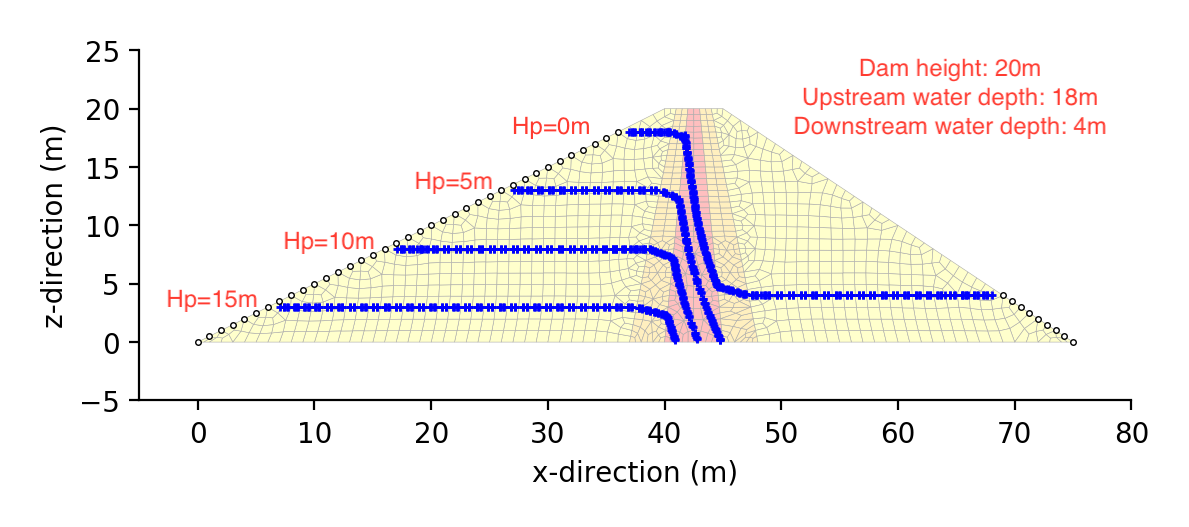
6.2 Outline of sample analysis model
Sample model is a zoned rock fill type dam which has height of 20m. In the sample analysis, a steady seepage flow analysis was carried out under the conditions shown below.
Height
(m) | Top width
(m) | Upstream
slope | Downstream
slope | Upstream
water depth (m) | Downstream
water depth (m) |
|---|
| 20.0 | 5.0 | 1:2.0 | 1:1.5 | 18.0 | 4.0 |
| Material properties |
|---|
| Zone | Permeability
k (m/s) | α
(m$^{-1}$) | m |
|---|
| Upstream shell | 1 x 10$^{-2}$ | 0.1 | 0.7 |
| Upstream filter | 1 x 10$^{-5}$ | 0.1 | 0.7 |
| Center core | 1 x 10$^{-6}$ | 0.1 | 0.7 |
| Downstream filter | 1 x 10$^{-5}$ | 0.1 | 0.7 |
| Downstream shell | 1 x 10$^{-2}$ | 0.1 | 0.7 |
6.3 Execution command for FEM analysis and drawing
python3 py_fem_seep4.py inp_zone4.txt out_zone4.txt
python3 py_seep4_cont.py out_zone4.txt
python3 py_seep4_vect.py out_zone4.txt
| inp_zone4.txt | : FEM analysis input data (separated by space) |
| out_zone4.txt | : FEM analysis output data (separated by space) |
In the drawing program 'py_seep4_cont.py', a image file named '_fig_seep4_cont.png' is created automatically. Although the drawing range is set automattically, the contour pitch of pressure head shall be amended considering the result of the analysis.
In the drawing program 'py_seep4_vect.py', a image file named '_fig_seep4_vect.png' is created automatically.
6.4 Sample drawings
(1) Simple pressure head contour
A png image which was drawn using a program 'py_seep_cont.py' is shown below.
Pressure head values (Hp=0m,5m,10m,15m) which are shown using red color character and some information shown in upper-right location are added later using Mac application of 'Preview'. (Preview $\rightarrow$ Tools $\rightarrow$ Annotate $\rightarrow$ Text)
(Notice) In the actural zoned rockfill type dam, it is already known that the sudden pressure head drop in the core zone has not been observed and the phenomena of pressure drop has been observed along the boundary of the core zone and filter zone. Please understand that this analysis is only a sample for the test of program functions.
(2) Velocity vector diagram
A png image which was drawn using a program 'py_seep_vect.py' is shown below.
Mean velocity vectors for saturated elements are shown using 'Navy' color, and mean velocity vectors for unsaturated elements are shown using 'Magenta' color.
Although it is simple and convenient to use a matplot command 'quiver' for vector plotting, 'plot' command is used in this program because of some troubles in the drawing work.
2D Thermal Conductivity Analysis
1. Outline
- This is a program for 2D unsteady thermal conductivity analysis with isotropic material. This program can not treat steady ot anisotropic material problem.
- Thickness of the element is unit thickness and it is not changeable.
- As boundary conditions, thermal insulation boundary, temperature given boundary and heat transfer boundary can be considered.
- Heating material such as cement concretecan also be used .
- 4 node isoparametric element with 4 Gauss points is used. 1 node has 1 degree of freedom of temperature or heat flux.
- In coordinate system, x-direction is defined as right-direction and y-direction is defined as upward direction.
- Crank-Nicolson method is used for the discretization of the time.
- Simultaneous linear equations are solved using numpy.linalg.inv(A).
Although this solving process has repeating process for time history analysis, matrix for calculation is not changed if the time increment is not changed.
Therefore, to calculate an inverse matrix is carried out only one time, and it is used to calculate the time history of the temperature until the end of the calculation time.
- Input/Output file name can be defined arbitrarily with the format of space separater and those are inputted as command line arguments of a terminal.
In addition, it is necessary to prepare the input file for time history of node temperatures of given temperature boundary and side temperatures of heat transfer boundary.
| Valid boundary conditions |
|---|
| Item | Description |
|---|
| Thermal insulation boundary | No input means thermal insulation boundary |
| Temperature given boundary | Specify the nodes and time history of temperature at specified nodes |
| Heat transfer boundary | Specify the sides of element, heat transfer coefficient and time history of temperature at outside |
Supplemrntal explanation of heating material
Heating material can be used like a cement concrete.
Properties of heating materials are inputted as element material characteristics.
In this program, heat generation of cement concrete is imitated and the adiabatic temperature rise shown below formula can be considered.
\begin{equation}
T=K\cdot(1-e^{-\alpha\cdot t})
\end{equation}
where, $T$: adiabatic temperature rise, $K$: maximum temperature rise, $\alpha$: coefficient of heat release rate, $t$: time.
In this program, $K$ (Tk) and $\alpha$ (Al) become input data and heat generation rate per unit area is calculated in calculation process.
Supplemental explanation of heat transfer boundary
It is necessary for heat transfer boundary to be defined as a side of an element.
Therefore, element number and one node which forms a heat transfer boundary shall be inputted as input data.
Since the node numbers which forms an element are inputted with the sequence of counterclockwise in FEM input data, the side can be identified by specifying a first node of the side with heat transfer boundary.
2. FEM program
| Program name | Description |
|---|
| py_fem_heat.py | 2D Thermal Conductivity Analysis program |
3. Command format for FEM analysis execution
python3 py_fem_heat.py inp1.txt inp2.txt out.txt
| inp1.txt | : First input data file for analysis model (separated by space) |
| inp2.txt | : Second input data file for time histories of temperature given nodes or outside temperature of heat transfer boundary (separated by space) |
| out.txt | : Output data file (separated by space) |
4. Input data format
(1) Analysis model data
npoin  nele  nsec  kot  koc  delta    # Basic values for analysis
Ak  Ac  Arho  Tk  Al                  # Material properties
     ..... (1 to nsec) .....          #
node-1  node-2  node-3  node-4  isec  # Element connectivity, Material set number
     ..... (1 to nele) .....          #   (counterclockwise order of node numbers)
x  y  T0                              # Coordinates of node, initial temperature of node
     ..... (1 to npoin) .....         #   (x: right-direction, y: upward direction)
nokt                                  # Node number of temperature given boundary
     ..... (1 to kot) .....           #   (Omit data input if kot=0)
nekc_0  nekc_1  alphac                # Element number, node number defined side, heat transfer rate
     ..... (1 to koc) .....           #   (Omit data input if koc=0)
n1out                                 # Number of nodes for output of temperature time history
n1node_1  ..... (1 line input) .....  # Node number for above
n2out                                 # frequency of output of temperatures of all nodes
n2step_1  ..... (1 line input) .....  # Time step number for above (Omit data input if ntout=0)
| npoin, nele, nsec | : number of nodes, number of elements, number of material sets |
| kot, koc | : number of temperature given nodes, number of heat transfer boundary sides |
| delta | : time increment |
| Ak, Ac, Arho | : heat conductivity coefficient, specific heat, unit weight |
| Tk, Al | : maximum temperature rise, coefficient of heat release rate (for heating material) |
| x, y, T0 | : x and y coordinates, initial temperature of node |
| nokt | : node with temperature given boundary |
| nekc_0, nekc_1, alphac | : element and first node with heat transfer boundary side, heat transfer rate |
| n1out | : number of nodes for all time history output |
| n1node | : node numbers for all time history output |
| n2out | : number of steps for all nodes temperature output |
| n2step | : step numbers for all nodes temperature output |
(2) Time history data for temperature given nodes or heat transfer boundary sides
   1   TE[1] ... TE[kot] TC[1] ... TC[koc]   # data of 1st time step
   2   TE[1] ... TE[kot] TC[1] ... TC[koc]   # data of 2nd time step
   3   TE[1] ... TE[kot] TC[1] ... TC[koc]   #
    ..... (repeating until end time) .....   #
itime  TE[1] ... TE[kot] TC[1] ... TC[koc]   #
| kot | : number of nodes with temperature given boundary |
| koc | : number of sides with heat transfer boundary |
| TE[1~kot] | : temperature time history at temperature given boundary node |
| TC[1~koc] | : time history of outside temperature at heat transfer boundary side |
5. Output data format
npoin  nele  nsec  kot  koc  delta  niii  n1out  n2out
    (Each value of above)
sec  Ak  Ac  Arho  Tk  Al
    sec  : Material number
    Ak   : Heat conductivity coefficient
    Ac   : Specific heat
    Arho : Unit weight
    Tk   : Maximum temperature rize
    Al   : Heat release rate
    ..... (1 to nsec) .....
node  x  y  tempe0  Tfix
    node   : Node number
    x      : x-ccordinate
    y      : y-coordinate
    tempe0 : Initial temperature
    Tfix   : Index of node with given temperature (0: free, 1: fixed)
    ..... (1 to npoin) .....
nek0  nek1  alphac
    nek0   : Element number with heat transfer boundary
    nek1   : Node number to specify heat transfer boundary side of an element
    alphac : Heat transfer rate at the specified side of an element
    ..... (1 to koc) .....
elem  i  j  k  l  sec
    elem : Element number
    i    : Node number of start point
    j    : Node number of second point
    k    : Node number of third point
    l    : Node number of end point
    sec  : Material number
    ..... (1 to nele) .....
iii  ttime  Node_(xx)  Node_(xx)  Node_(xx) .....
    iii       : Time step
    ttime     : Time
    Node-(xx) : Node number
    Time historis of each node temperature are written.
    ..... (0 to end of calculation time) .....
node  t=0.0  t=(xx)  t=(xx)0  t=(xx) .....
    node   : Node number
    t=(xx) : Specified time
    Node temperatures at specified time are written.
    ..... (1 to npoin) .....
n=(total degrees of freedom)  time=(calculation time)
6. Output sample
6.1 Input data sample and auxiliary program
| Program name | Description |
|---|
| inp_div20_model.txt | First FEM analyis input data (analysis model data) |
| inp_div20_thist.txt | Second FEM analysis input data (temperature time history for specified nodes or sides) |
| py_heat_2D.py | Drawing program of temperature time history (matplotlib) |
| py_heat_3D.py | 3D drawing program of temperature distribution at specified time (GMT) |
6.2 Outline of sample analysis model
Model shape is a square with 1m length side and inside element is formed by heating material. 4 sides of the model has heat transfer boundary. Material properties and analysis conditions are shown below.
| Characteristics of model |
|---|
| Heat conductivity coefficient | 2.5 kcal/m h $^{\circ}$C |
| Specific heat | 0.28 kcal/kg $^{\circ}$C |
| Unit weight | 2350 kg/m$^3$ |
| Heat transfer rate | 10 kcal/m$^2$ h $^{\circ}$C |
Adiabatic temperature raise
(heating material) | $T=K\cdot(1-e^{-\alpha t})$, K=40$^{\circ}$C, α=0.2, t: hour |
| Model | 1m square area, 441 nodes, 400 elements |
| Conditions for analysis |
|---|
| Initial temperature of domain | 20 $^{\circ}$C for all nodes |
| Boundary condition | 4 sides have heat transfer boundary with outside temperature of 10 $^{\circ}$C |
| Heat generation of elements | Considered for all elements |
6.3 Execution command for FEM analysis and drawing
python3 py_fem_heat.py inp_div20_model.txt inp_div20_thist.txt out_div20.txt

python3 py_heat_2D.py out_div20.txt

python3 py_heat_3D.py out_div20.txt
bash _a_gmt_3D.txt
mogrify -trim -density 300 -bordercolor 'transparent' -border 10x10 -format png *.eps
rm *.eps
| inp_div20_model.txt | : First FEM analysis input data of modeling (separated by space) |
| inp_div20_thist.txt | : Second FEM analysis data of temperature time histories (separated by space) |
| out_div20.txt | : FEM analysis output data (separated by space) |
| _a_gmt_3D.txt | : GMT script by 'py_heat_3D.py' |
Program 'py_heat_2D.py'
Program 'py_heat_2D.py' creates a image file of '_fig_tem_his.png' aotomatically.
Program 'py_heat_3D.py'
- This program creates a GMT (Generic Mapping Tools) script named '_a_gmt_3D.txt' automatically.
- By execution of above GMT script, eps image files named '_fig_gmt_xyz_0.eps', '_fig_gmt_xyz_1.eps', .... are created automatically.
- In above execution command, eps image files by GMT are converted to png image files using ImageMagick command 'mogrify'.
6.4 Sample drawing
(1) Temperature time histories at specified nodes
A image created by 'py_heat_2D.py' is shown below.
(2) 3D temperature distributions at specified step
A image created by 'py_heat_3D.py' and GMT is shown below. Below image is created by integration of 8 image files using TeX and ImageMagick. Unit of 't' in below image is 'hours'.
2D Frame Vibration Analysis
1. Outline
(1) Time history response analysis
- This is a program for 2D frame time history response analysis with elastic material and small displacement theorey
- Beam element with 2 nodes is used. 1 node has 3 degrees of freedom in horizontal displacement, vertical displacement and rotation.
- Nodal external force can be given as a rate load, and only one acceleration time history can be given.
Actually, the product of nodal external unit forces and acceleration becomes the loads to structure.
- In coordinate system, x-direction is defined as right-direction, y-direction is defined as upward direction and counterclockwise direction is defined as positive in rotation.
- Simultaneous linear equations are solved using numpy.linalg.inv(A).
Although this solving process has repeating process for time history analysis, matrix for calculation is not changed if the time increment is not changed.
Therefore, to calculate an inverse matrix is carried out only one time, and it is used to calculate the time history response until the end of the calculation time.
- Input/Output file name can be defined arbitrarily with the format of space separater and those are inputted as command line arguments of a terminal.
In addition, it is necessary to prepare the input file for acceleration time history.
| Valid boundary conditions |
|---|
| Item | Description |
|---|
| External force | Specify the loded nodes and rate load values |
| Forced displacement | Specify the nodes with fixed conditions. Only perfect fixed condition (zero displacement) can be treated |
(2) Eigenvalue analysis
- This is a program for 2D frame vibration eigen value analysis with elastic material and small displacement theorey
- Beam element with 2 nodes is used. 1 node has 3 degrees of freedom in horizontal displacement, vertical displacement and rotation.
- In coordinate system, x-direction is defined as right-direction, y-direction is defined as upward direction and counterclockwise direction is defined as positive in rotation.
- Characteristic equation are solved using w,vr=scipy.linalg.eig(K, M) as a generalized eigenvalue problem
- Input/Output file name can be defined arbitrarily with the format of space separater and those are inputted as command line arguments of a terminal.
| Valid boundary conditions |
|---|
| Item | Description |
|---|
| Forced displacement | Specify the nodes with fixed conditions. Only perfect fixed condition (zero displacement) can be treated |
2. FEM program
| Filename | Description |
|---|
| py_fem_vfrm.py | 2D frame time history response analysis program |
| py_fem_efrm.py | 2D frame vibration eigenvalue analysis program |
3. Command format, input and output data format for time history response analysis program
3.1 Command format for FEM analysis execution
Two input files are required for this program. One is for structural model data, another is for acceleration time history data.
python3 py_fem_vfrm.py inp1.txt inp2.txr out.txt
| inp1.txt | : First input data for structural model (separated by space) |
| inp2.txt | : Second input data including acceleration time history (separated by space) |
| out.txt | : Output data file (separated by space) |
3.2 Input file format
(1) First input data for structural model
npoin  nele  nsec  npfix  nlod                   # Basic values for analysis
E  A  I  gamma  zeta_m  zeta_k                   # Material properties
    ..... (1 to nsec) .....                      #
node_1  node_2  isec                             # Element connectivity, material set number
    ..... (1 to nele) .....                      #
x  y                                             # Node coordinate
    ..... (1 to npoin) .....                     #
lp  fix_x  fix_y  fix_r                          # Restricted node and restrict conditions
    ..... (1 to npfix) .....                     #
lp  fp_x  fp_y  fp_r                             # Loaded node and loading conditions
    ..... (1 to nlod) .....                      #     (omit data input if nlod=0)
| npoin, nele, nsec | : number of nodes, number of elements, number of material sets |
| npfix, nlod | : number of restricted nodes, number of loaded nodes |
| E, A, I, gamma | : elastic modulus, section area, moment of inertia, unit weight |
| zeta_m, zeta_k | : coefficients of Rayleigh damping |
| node_1, node_2, isec | : nodes forms an element, material set number |
| x, y | : x and y coordinates |
| lp, fix_x, fix_y, fix_r | : node, kind of restriction in x, y-direction and rotation, (0: free, 1: fixed) |
| lp, fp_x, fp_y, fp_r | : loaded node, loading rate in x, y-direction and rotation |
(2) Second input data including acceleration time history
delta      # time increment (sec)
acc1       # start of acceleration data
acc2
acc3
....
(until end of data)
3.3 Output data format
npoin  nele  nsec  npfix  nlod  ndoutx  ndouty  nfout  delta  nnn
    (Each value of above)
sec  E  A  I  gamma  zeta_m  zeta_k
    sec    : Material number
    E      : Elastic modulus
    A      : Section area
    I      : Moment of inertia
    gamma  : Unit weight
    zeta_m : Coefficient of Rayleigh damping for mass matrix
    zeta_k : Coefficient of Rayleigh damping for stiffness matrix
    ..... (1 to nsec) .....
node  x  y  fx  fy  fr  kox  koy  kor
    node   : Node number
    x      : x-coordinate
    y      : y-coordinate
    fx     : Load in x-direction
    fy     : Load in y-direction
    fr     : Moment load
    kox    : Index of restriction in x-direction (0: free, 1: fixed)
    koy    : Index of restriction in y-direction (0: free, 1: fixed)
    kor    : Index of restriction in rotation    (0: free, 1: fixed)
    ..... (1 to npoin) .....
elem  i  j  sec
    elem : Element number
    i    : Node number of start point
    j    : Node number of end point
    sec  : Material number
    ..... (1 to nele) .....
step  time  acc_inp  dis_x(ii) vel_x(ii) acc_x(ii)  Ni(ne)node  Si(ne)  Mi(ne)
    step      : Time step
    time      : Time
    acc_inp   : Input acceleration
    dis_x(ii) : Displacement in x-direction at node-ii
    vel_x(ii) : Velocity in x-direction at node-ii
    acc_x(ii) : Acceleration in x-direction at node-ii
    Ni(ne)    : Axial force at node-i in element-ne
    Si(ne)    : Shear force at node-i in element-ne
    Mi(ne)    : Moment at node-i in element-ne
    ..... (to end of time step) .....
n=(total degrees of freedom)  time=(calculation time)
| time, acc_inp | : time, input acceleration |
| dis, vel, acc | : displacement, velocity, acceleration |
| N, S, M | : axial force, shearing force, moment |
| n | : Total degrees of freedom (the number of the variables) |
| time | : Calculation time |
4. Command format, input and output data format for vibration eigenvalue analysis program
4.1 Command format for FEM analysis execution
python3 py_fem_efrm.py inp.txt out.txt
| inp.txt | : FEM analysis input data (separated by space) |
| out.txt | : FEM analysis output data (separated by space) |
4.2 Input data format
npoin  nele  nsec  npfix         # Basic values for analysis
E  A  I  gamma                   # Material properties
    ..... (1 to nsec) .....      #
node_1  node_2  isec             # Element connectivity, material set number
    ..... (1 to nele) .....      #
x  y                             # Node coordinate
    ..... (1 to npoin) .....     #
lp  fix_x  fix_y  fix_r          # Restricted node and restrict conditions
    ..... (1 to npfix) .....     #
| npoin, nele, nsec, npfix | : number of nodes, number of elements, number of material sets, number of restricted nodes |
| E, A, I, gamma | : elastic modulus, section area, moment of inertia, unit weight |
| node_1, node_2, isec | : nodes forms an element, material set number |
| x, y | : x and y coordinates |
| lp, fix_x, fix_y, fix_r | : node, kind of restriction in x, y-direction and rotation, (0: free, 1: fixed) |
4.3 Output data format
npoin  nele  nsec  npfix
    (Each value of above)
sec  E  A  I  gamma
    sec    : Material number
    E      : Elastic modulus
    A      : Section area
    I      : Moment of inertia
    gamma  : Unit weight
    ..... (1 to nsec) .....
node  x  y  kox  koy  kor
    node   : Node number
    x      : x-coordinate
    y      : y-coordinate
    kox    : Index of restriction in x-direction (0: free, 1: fixed)
    koy    : Index of restriction in y-direction (0: free, 1: fixed)
    kor    : Index of restriction in rotation    (0: free, 1: fixed)
    ..... (1 to npoin) .....
elem  i  j  sec
    elem : Element number
    i    : Node number of start point
    j    : Node number of end point
    sec  : Material number
    ..... (1 to nele) .....
Order         1       2       3  ......
fn(Hz)      w[1]   w[2]    w[3]  ......
v[  1]   v[1,1]  v[1,2]  v[1,3]  ......
v[  2]   v[1,1]  v[1,2]  v[1,3]  ......
......   ......  ......  ......  ......
v[  n]   v[1,1]  v[1,2]  v[1,3]  ......
    Order  Ranking
    w[i]      : Natural frequency (eigen value)
    v[j,i]    : Element of eigen vector
n=(total degrees of freedom)  time=(calculation time)
(Notice)
Regarding the treatment of restricted nodes in this eigenvalue analysis, since the degrees of freedom is not changed and the number of variables is kept for eigen value calculation, the eigenvalues equivalent to restricted degrees of freedom are concentrated to small value side and they have the same values by small order sorting.
And eigen vector equivalent to restricted degrees of freedom has special values which is formed only one and zero.
Using this character, the eigenvalues and eigen vectors equivalent to restricted degrees of freedom are not written in the output file.
Following is a sample of sorting result of eigenvalues.
[  1.59154943e-01   1.59154943e-01   1.59154943e-01   1.59154943e-01
   1.59154943e-01   1.59154943e-01   1.59154943e-01   1.59154943e-01
   1.59154943e-01   1.59154943e-01   1.59154943e-01   1.59154943e-01
   1.59154943e-01   2.35776685e+00   1.47763490e+01   4.13833696e+01
   8.11515057e+01   1.34359374e+02   2.01285622e+02   2.82413495e+02
   3.78356230e+02   4.89209902e+02   6.08158484e+02   8.09431960e+02
   9.77895783e+02   1.18543706e+03   1.43074344e+03   1.71924912e+03
   2.05623517e+03   2.44043231e+03   2.84908857e+03   3.20838993e+03
   4.01526229e+03]
5. Output sample (Gauss wave input)
5.1 Auxiliary program
| Program name | Description |
|---|
| py_fig_vfrm.py | Drawing program for response time history and Fourier spectra (matplotlib) |
| py_gauss.py | Program for Gauss wave creation (max. 100gal) |
| py_im.py | Text addition program to image file using ImageMagick |
| py_fn_canti.py | Program for natural frequency calculation of cantilever using scipy |
| py_fig_efrm_mode.py | Drawing program of natural vibration mode (matplotlib) |
Drawing program for response time history and Fourier spectra (py_fig_vfrm.py)
- Drawings of response time histories of node acceleration, velocity, displacement and section forces can be created using matplotlib.
- Drawings of Fourier spectra of node acceleration, velocity, displacement and section forces can be created using matplotlib. For the First Fourier Transform, numpy.fft is used.
- For search of dominant frequency (natural frequency), scipy.argrelmax(sp0,order=100) is used, where 'sp0' means Fourier spectrum by fft, 'order=100' means a parameter to search the local maximum.
Program for Gauss wave creation (py_gauss.py)
- Gauss wave can be created using the time increment inputted from command line.
- Gauss wave has the characteristics of average=0.5sec, standard deviation=0.001 and maximum acceleration=100gal.
Text addition program to image file using ImageMagick (py_im.py)
- The purpose of this program is to add some text to existing png image file.
- Although this is Python program, ImageMagick command is used for actural processing through 'os.system(cmd)'.
Program for natural frequency calculation of cantilever using scipy (py_fn_canti.py)
- Since it is necessary to solve a nonlinear equation $\cos x \cdot \cosh x + 1 =0$ for calculation of cantilever batural frequency, scipy.optimize.brentq is used for this work.
- Since it is clear for above nonlinear equation to have periodic solutions between 0〜π π〜2π ... , initial values for brentq are set considering this characteristics.
Drawing program of natural vibration mode (py_fig_efrm_mode.py)
- Natural vibration mode diagrams can be created from eigenvalue analysis results using matplotlib.
5.2 Outline of sample analysis model
The sample model is a vertical cantilever which has fixed base and is subjected to horizontal ground acceleration.
Although a ground acceleration acts on the base, all nodes are subjected to the acceleration because base is completely fixed.
5.3 Input data
(1) Structural model data
This is a vertical cantilever with completely fixed base. The unit of dimensions and material properties is under m-system.
The load values are rates which are multiplied to ground acceleration.
If the unit od ground acceleration is gal (cm/s^2), loading rate should be 0.01, because the unit of structural dimension is fixed to m-system (gravity acceleration $g=9.8m/s^2$).
11  10  1  1  11                    # Basic data
2000000  0.25  0.005208  2.3  0  0  # E  A  I  gamma  zeta_m  zeta_k
 1   2  1                           # Element-node relationship, material No.
 2   3  1                           #
 3   4  1                           #
 4   5  1                           #
 5   6  1                           #
 6   7  1                           #
 7   8  1                           #
 8   9  1                           #
 9  10  1                           #
10  11  1                           #
0  0                                # x, y-coordimates
0  1                                #
0  2                                #
0  3                                #
0  4                                #
0  5                                #
0  6                                #
0  7                                #
0  8                                #
0  9                                #
0  10                               #
1  1  1  1                          # Node No, restrict conditions
 1  0.01  0  0                      # Node number and Loading condition
 2  0.01  0  0                      #
 3  0.01  0  0                      # In this case, all nodes are loaded
 4  0.01  0  0                      # in x-direction.
 5  0.01  0  0                      # The values 0.01 means the coefficient
 6  0.01  0  0                      # for the input acceleration.
 7  0.01  0  0                      # Since the unit of input acceleration
 8  0.01  0  0                      # is 'gal' (cm/s^2) usually,
 9  0.01  0  0                      # the coefficient should be 0.01
10  0.01  0  0                      # because the unit of structural dimensions
11  0.01  0  0                      # are 'm'
1                                   # Number of nodes for x-dir. output (ndoutx)
11                                  # Node for dis-vel-acc output
0                                   # Number of nodes for y-dir. output (ndouty)
1                                   # Number of nodes for section force output (nfout)
1  1                                # Element and node (node should be 1 or 2)
(2) Ground acceleration data
Data shown below was made by program 'py_gauss.py'. The wave is one of the Gauss wave which has average=0.5sec, maximum value of 100gal and time increment 0.01sec.
0.01                   # time increment (sec)
0.0                    # start of acceleration time history
0.0
0.0

......

3.69388306849e-194
1.38389652674e-85
1.92874984796e-20
100.0                 # 100 gal at t=0.5sec
1.92874984796e-20
1.38389652674e-85
3.69388306848e-194

......

0.0
0.0
0.0
5.4 Command for execution
- To make ground acceleration data using program 'py_gauss.py' with time increment 0.001sec.
- To carry out the time history response analysis using program 'py_fem_vfrm.py'.
- To create drawings of response time historis and Fourier spectra using program 'py_fig_vfrm.py'.
- To combine created images using ImageMagick command 'convert -append'.
#dt=0.001
python py_gauss.py 0.001 > inp_gauss.txt
python py_fem_vfrm.py inp_vfrm.txt inp_gauss.txt out_vfrm.txt
python py_fig_vfrm.py out_vfrm.txt

convert -append _fig_fft_acc_inp.png _fig_fft_acc_x\(11\).png _1.png
convert -append _1.png _fig_fft_vel_x\(11\).png _2.png
convert -append _2.png _fig_fft_dis_x\(11\).png _3.png
convert -append _3.png _fig_fft_S1\(1\).png _4.png
convert -append _4.png _fig_fft_M1\(1\).png fig_fft_001.png

convert -append _fig_his_acc_inp.png _fig_his_acc_x\(11\).png _1.png
convert -append _1.png _fig_his_vel_x\(11\).png _2.png
convert -append _2.png _fig_his_dis_x\(11\).png _3.png
convert -append _3.png _fig_his_S1\(1\).png _4.png
convert -append _4.png _fig_his_M1\(1\).png fig_his_001.png

#dt=0.005
python py_gauss.py 0.005 > inp_gauss.txt
python py_fem_vfrm.py inp_vfrm.txt inp_gauss.txt out_vfrm.txt
python py_fig_vfrm.py out_vfrm.txt

convert -append _fig_fft_acc_inp.png _fig_fft_acc_x\(11\).png _1.png
convert -append _1.png _fig_fft_vel_x\(11\).png _2.png
convert -append _2.png _fig_fft_dis_x\(11\).png _3.png
convert -append _3.png _fig_fft_S1\(1\).png _4.png
convert -append _4.png _fig_fft_M1\(1\).png fig_fft_005.png

convert -append _fig_his_acc_inp.png _fig_his_acc_x\(11\).png _1.png
convert -append _1.png _fig_his_vel_x\(11\).png _2.png
convert -append _2.png _fig_his_dis_x\(11\).png _3.png
convert -append _3.png _fig_his_S1\(1\).png _4.png
convert -append _4.png _fig_his_M1\(1\).png fig_his_005.png

#dt=0.01
python py_gauss.py 0.01 > inp_gauss.txt
python py_fem_vfrm.py inp_vfrm.txt inp_gauss.txt out_vfrm.txt
python py_fig_vfrm.py out_vfrm.txt

convert -append _fig_fft_acc_inp.png _fig_fft_acc_x\(11\).png _1.png
convert -append _1.png _fig_fft_vel_x\(11\).png _2.png
convert -append _2.png _fig_fft_dis_x\(11\).png _3.png
convert -append _3.png _fig_fft_S1\(1\).png _4.png
convert -append _4.png _fig_fft_M1\(1\).png fig_fft_010.png

convert -append _fig_his_acc_inp.png _fig_his_acc_x\(11\).png _1.png
convert -append _1.png _fig_his_vel_x\(11\).png _2.png
convert -append _2.png _fig_his_dis_x\(11\).png _3.png
convert -append _3.png _fig_his_S1\(1\).png _4.png
convert -append _4.png _fig_his_M1\(1\).png fig_his_010.png

rm _*
5.5 Input data for vibration eigenvalue analysis
Data for vibration eigenvalue analysis of vertical cantilever is shown below.
In an eigenvalue analysis, if the displacements in y-direction are not fixed, the obtained eigenvalues include some vertical vibration modes. Since only bending vibration modes are required in this sample analysis, the displacements in y-direction of all nodes are fixed.
11  10  1  11                 # npoin nele nsec npfix
2000000  0.25  0.005208  2.3  # Material properties
 1   2  1                     # Element-node relationship
 2   3  1                     #    and material number
 3   4  1                     #
 4   5  1                     #
 5   6  1                     #
 6   7  1                     #
 7   8  1                     #
 8   9  1                     #
 9  10  1                     #
10  11  1                     #
0  0                          # x, y-coordinate
0  1                          #
0  2                          #
0  3                          #
0  4                          #
0  5                          #
0  6                          #
0  7                          #
0  8                          #
0  9                          #
0  10                         #
1  1  1  1                    # Restrict conditions
2  0  1  0                    # Node-1: all are restricted
3  0  1  0                    #     because of fixed edge.
4  0  1  0                    # Node-2 to 11:
5  0  1  0                    #    y(horizontal)-direction are restricted
6  0  1  0                    #    becasu of to eliminate the effect of
7  0  1  0                    #    axial displacement.
8  0  1  0                    #
9  0  1  0                    #
10 0  1  0                    #
11 0  1  0                    #
5.6 Sample drawing
Structure is a vertical cantilever which has completely fixed base. Input acceleration wave is Gauss wave which has the characteristics that average=0.5sec, maximum accelerayion=100gal.
In the sample analysis, time increment is changed such as the value of dt=0.01, 0.005, 0.001sec.
(1) Response time history diagrams
| dt = 0.01 sec | dt = 0.005 sec | dt = 0.001 sec |
|---|
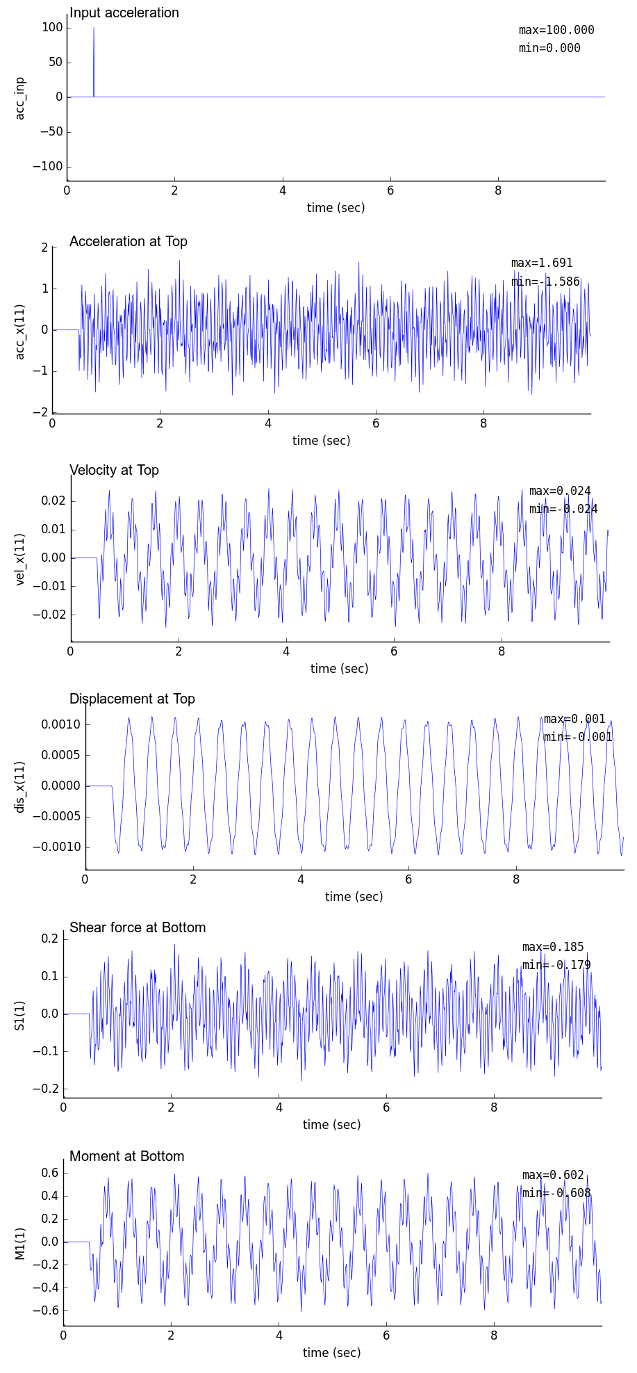 |
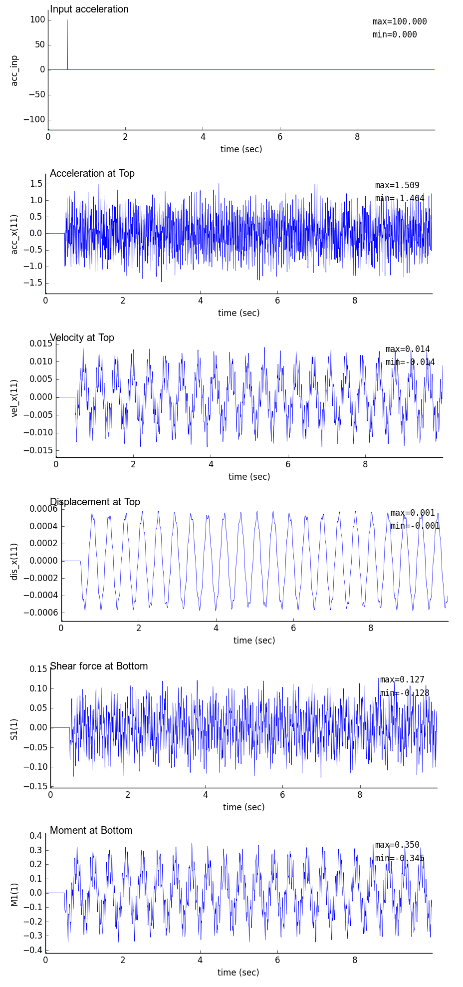 |
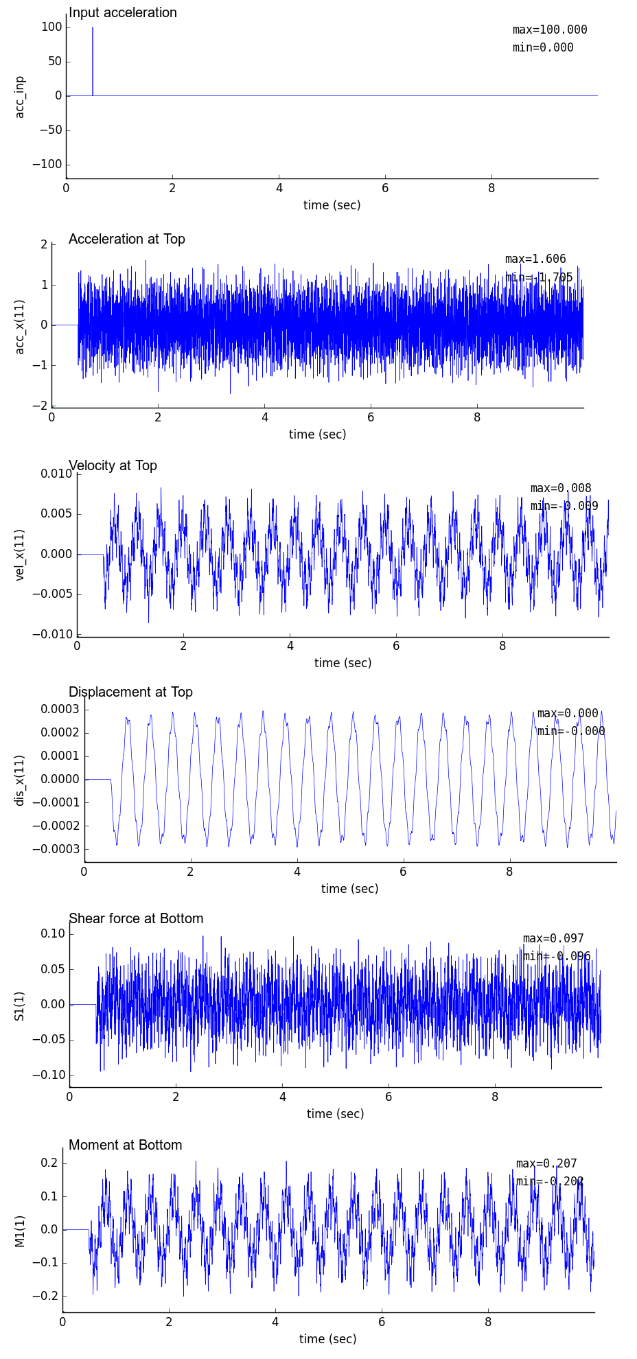 |
(2) Fourier spectrum diagrams
| dt = 0.01 sec | dt = 0.005 sec | dt = 0.001 sec |
|---|
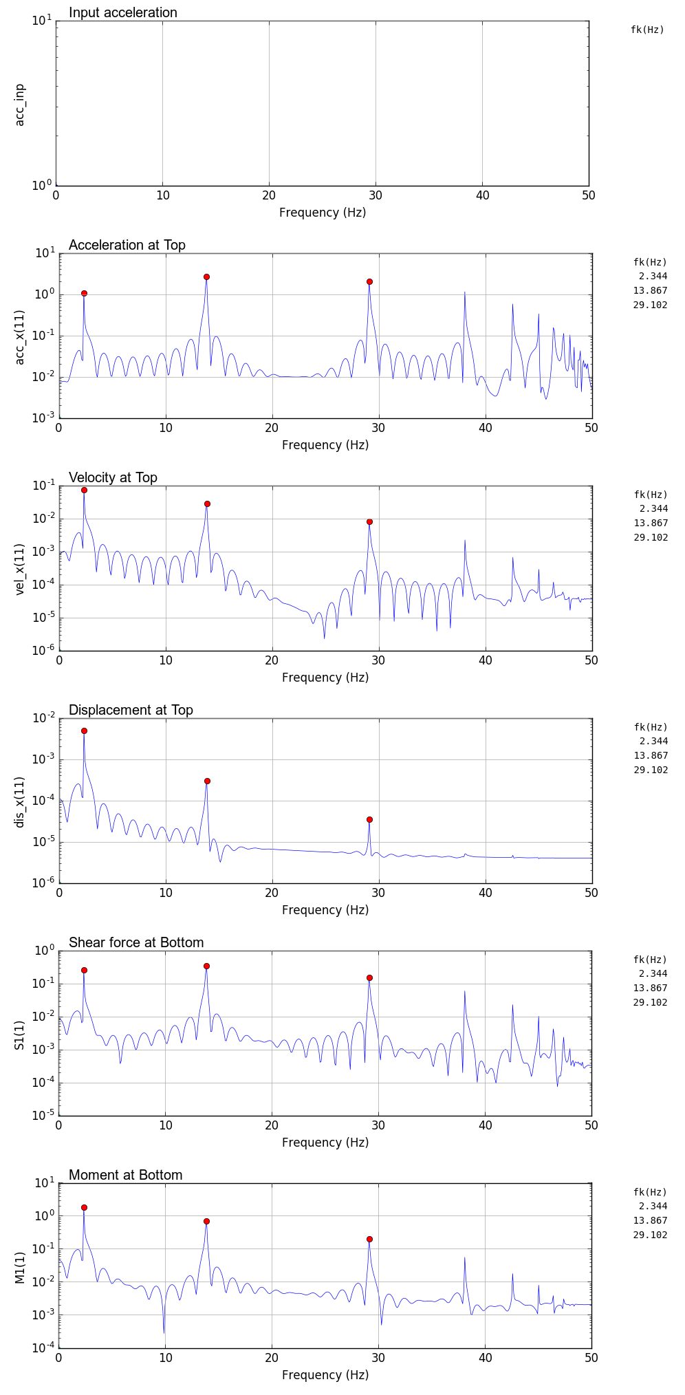 |
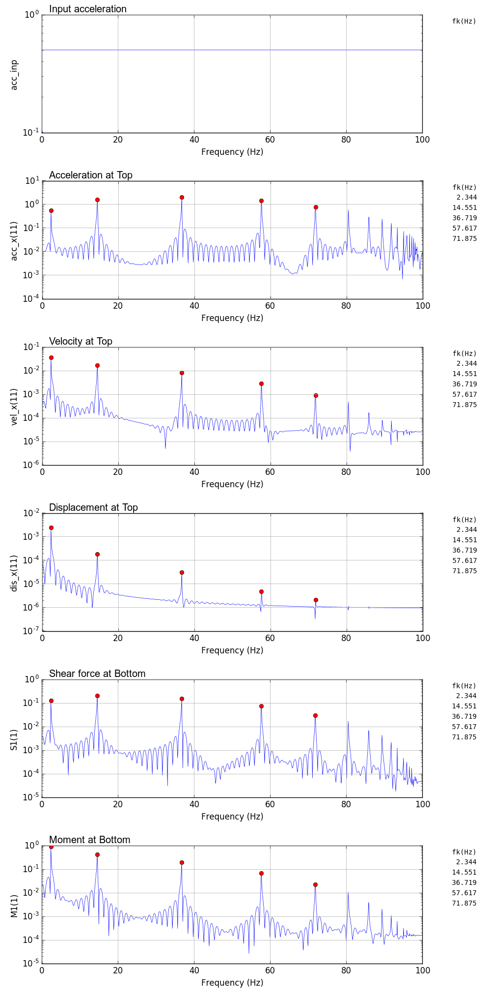 |
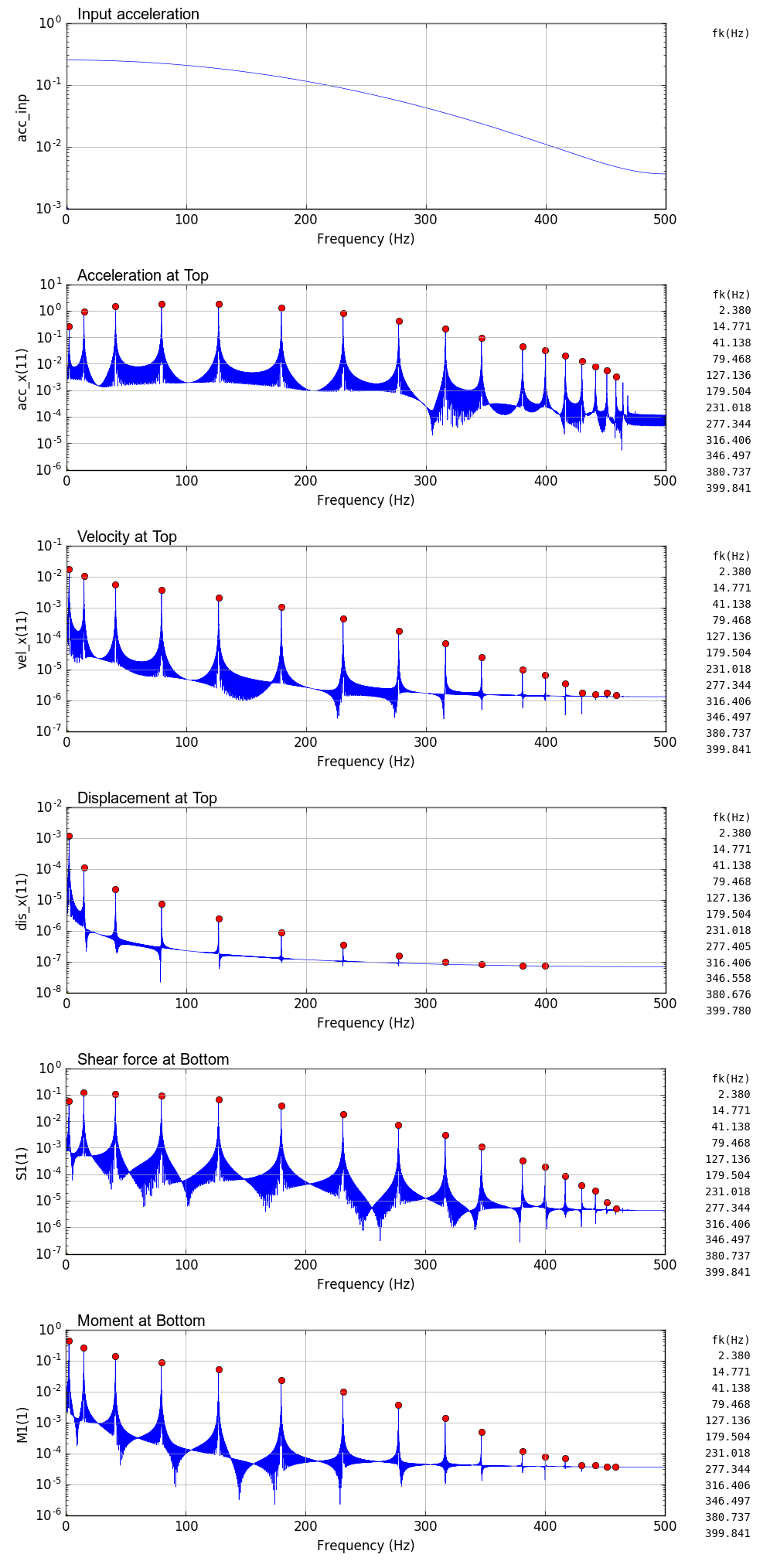 |
5.7 Comparison of natural frequency
The natural frequencies of vertical cantilever which were obtained from FEM analyses and those which were obtained from theoriticak calculations are shown below.
The shown natural frequencies from FEM analysis are the values obtained by use of scipy.argrelmax(sp0,order=100) (red circle in the drawings). In the FEM results, there are some peaks which are not searched by scipy.argrelmax. However, the natural frequencies in high frequensy range have no accuracy and they can not use as a characteristic of structure.
Comparison of natural frequency
| Theorem | Analysis results |
|---|
| mode | fn(Hz) | >Eigen value
Analysis | dt=
0.01s | dt=
0.005s | dt=
0.001s |
|---|
| 1 | 2.358 | 2.358 | 2.344 | 2.344 | 2.380 |
| 2 | 14.776 | 14.776 | 13.867 | 14.551 | 14.771 |
| 3 | 41.373 | 41.383 | 29.102 | 36.719 | 41.138 |
| 4 | 81.074 | 81.152 | | 57.617 | 79.468 |
| 5 | 134.022 | 134.359 | | 71.875 | 127.136 |
| 6 | 200.205 | 201.285 | | | 179.504 |
| 7 | 279.625 | 282.413 | | | 231.018 |
| 8 | 372.282 | 378.356 | | | 277.344 |
| 9 | 478.176 | 489.210 | | | 316.406 |
| 10 | 597.306 | 608.158 | | | 346.497 |
| 11 | 729.673 | 809.432 | | | 380.737 |
| 12 | 875.276 | 977.896 | | | 399.841 |
|
Valculation formula for cantilever natural frequency
\begin{equation}
f_n=\cfrac{1}{2\pi}\left(\cfrac{\alpha}{\ell}\right)^2 \sqrt{\cfrac{E I}{\rho A}}
\end{equation}
$\alpha$ shall satisfy following eqution.
\begin{equation}
\cos\alpha\cdot\cosh\alpha+1=0
\end{equation}
Material properties
$E=2,000,000 ~t/m^2$
$A=0.25 ~m^2$
$I=0.005208 ~m^4$
$\gamma=2.3 ~t/m^3$ ($\rho=\gamma~/~g~:~g=9.8m/s^2$)
$\ell=10 ~m$
|
| Vibration mode by eigenvalue analysis |
|---|
 |
6. Output sample (random wave input)
The shown case is that a vertical cantilever is subjected to horizontal random acceleration with the range of $\pm 1 gal$. The time increment was set to 0.001sec and the condition of local maximum search was set to 'order=200' [ maxID=argrelmax(sp0,order=200) ].
| Response time history (dt = 0.001 sec) | Fourier spectrum (dt = 0.001 sec) |
|---|
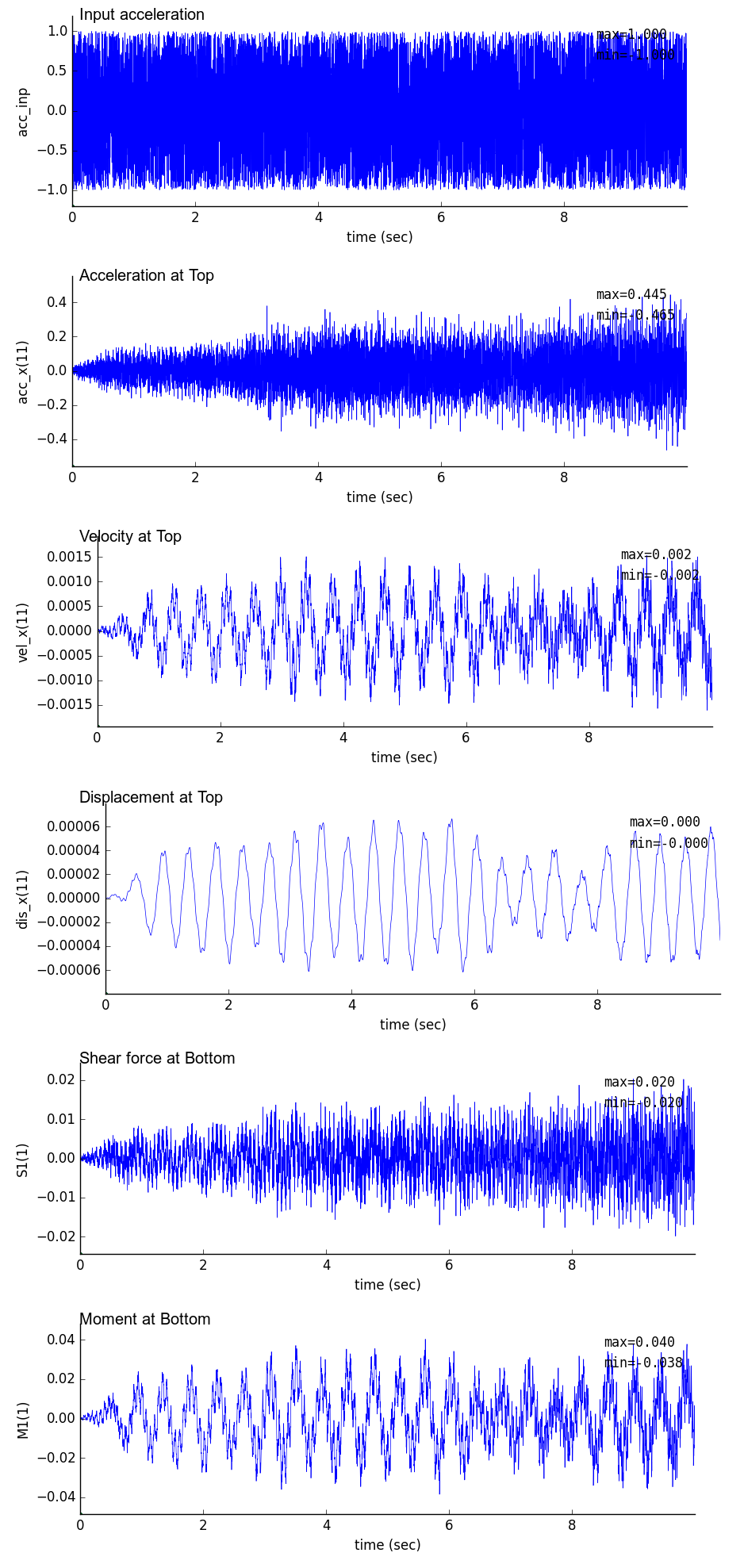 |
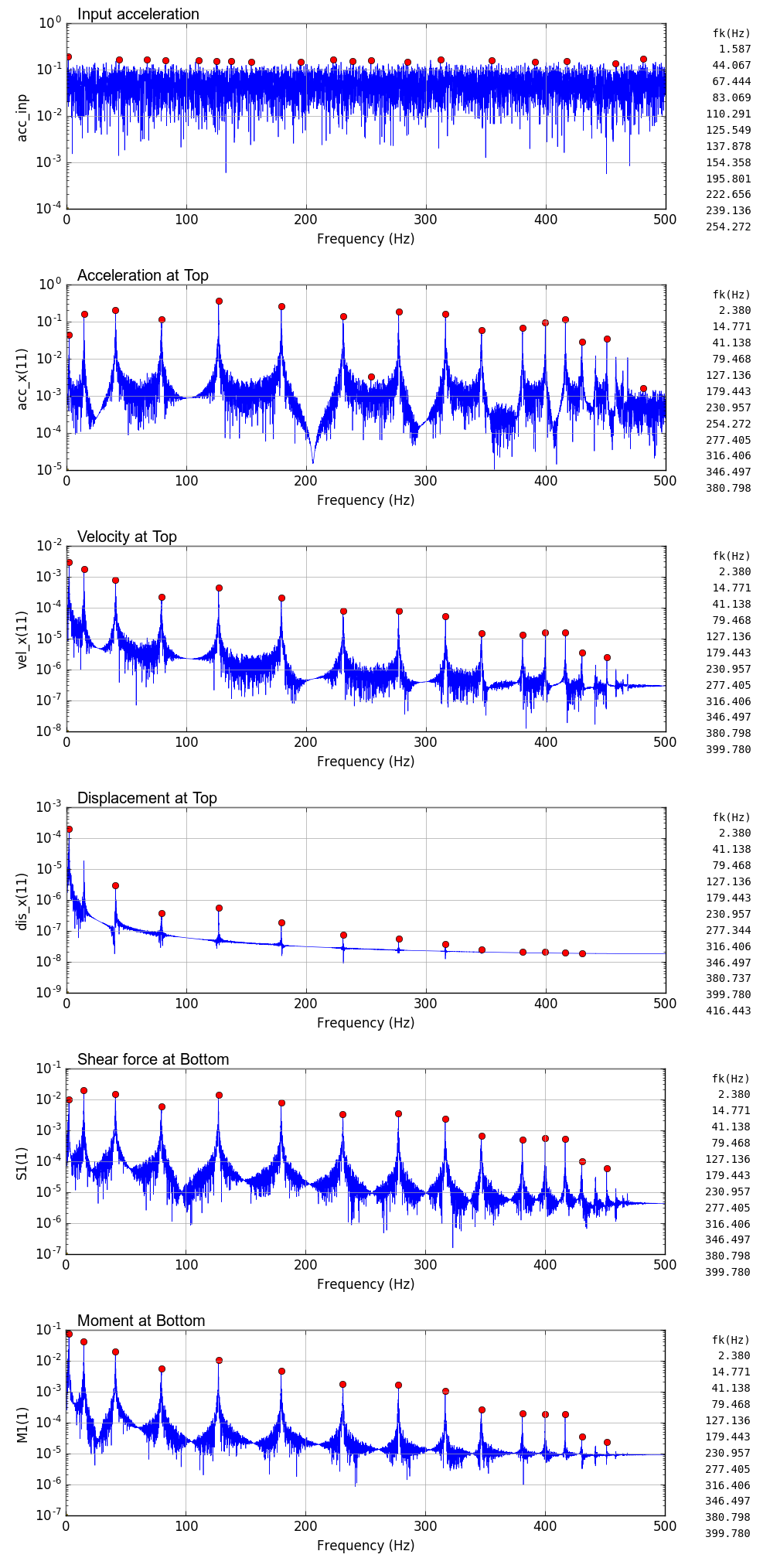 |
7. Output sample (Gauss wave, damping considered)
The shown case is that a vertical cantilever is subjected to horizontal Gauss wave acceleration with the maximum 100gal.
Damping characteristics of structure was calculated as follow. The 1st and 2nd natural frequency which were obtained from FEM eigenvalue analysis is used for following calculation.
| Mode | fn(Hz) | h | $\zeta$ |
|---|
| 1 | 2.358 | 0.05 | $\zeta_m$=1.2777 |
| 2 | 14.776 | 0.05 | $\zeta_k$=0.00092888 |
| Only $\zeta_m$ considered | Only $\zeta_k$ considered | Both of $\zeta_m$ and $\zeta_k$ considered |
|---|
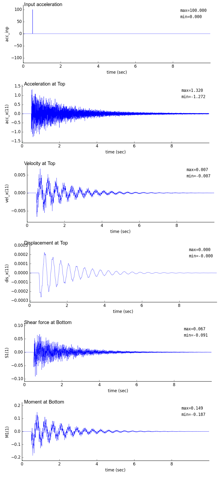 |
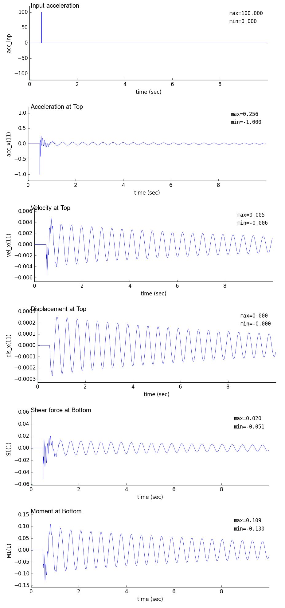 |
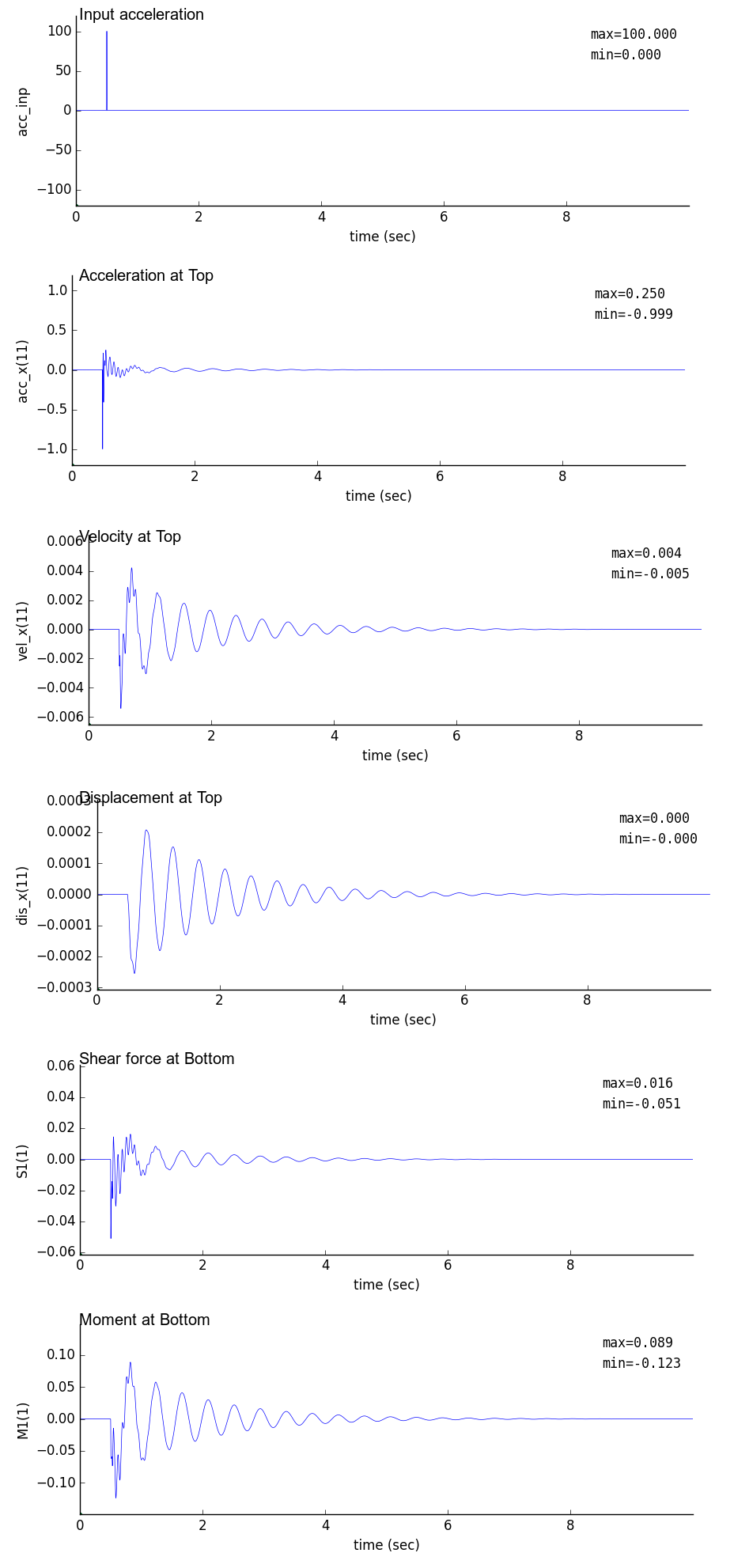 |
| Only $\zeta_m$ considered | Only $\zeta_k$ considered | Both of $\zeta_m$ and $\zeta_k$ considered |
|---|
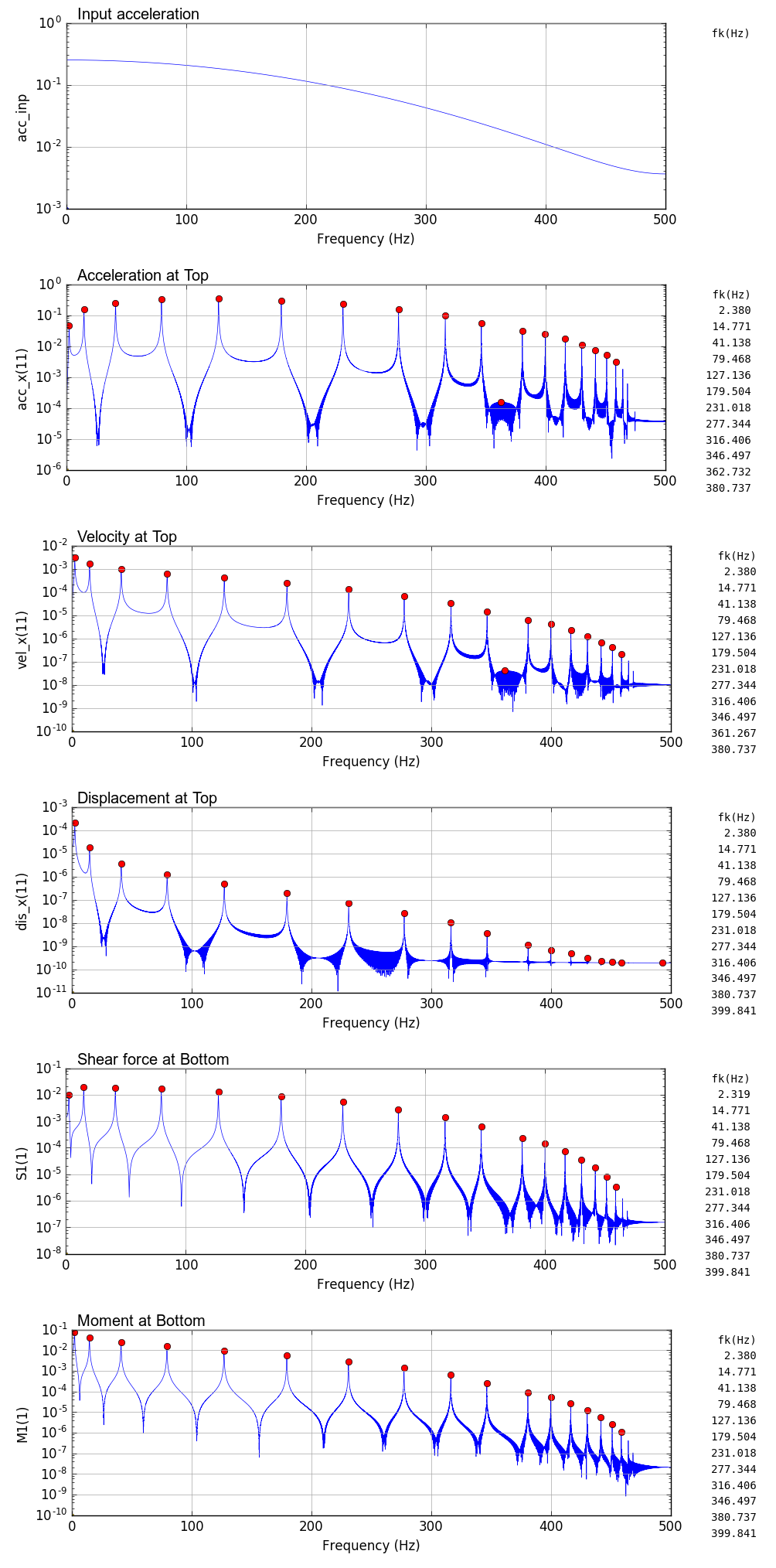 |
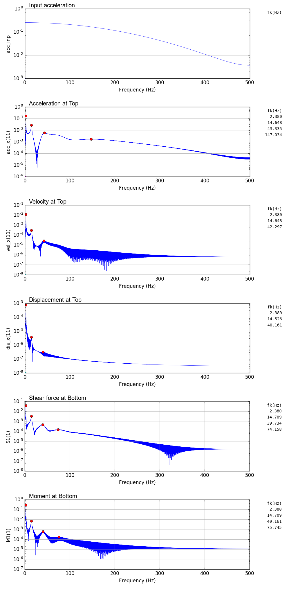 |
 |
8. Output sample (Earthquake wave, damping considered)
The case is that a vertical cantilever considered damping ($\zeta_m$ and $\zeta_k$) is subjected to the observed horizontal earthquake acceleration.
The coefficients for damping are the same as previous ones.
Two cases of time increment for analysis were considered.
One was dt=0.01sec which is the same as the sampling pitch od eartquake wave, another was dt=0.001sec for which the observed earthquake wave was amended by linear interpolation.
For the search of local maximum of frequency, 'order=1000' for scipy.argrelmax was used [ maxID=argrelmax(sp0,order=1000) ].
The linear interpolation program is shown below. In this program, scipy.interpolate is used.
Although there are 30,000 points in the original observed wave, the data from 5,000 to 25,001 was used for sample analysis.
import numpy as np
import matplotlib.pyplot as plt
from scipy import interpolate

data = np.loadtxt("test_eq010.txt")
x0=data[5000:25001]
dt=0.01
t0=np.arange(0, 200+dt, dt)
print(len(t0), len(x0))

plt.plot(t0,x0)
plt.show()

f = interpolate.interp1d(t0, x0)
dt=0.001
t1=np.arange(0, 200, dt)
x1 = f(t1)
print(len(t1), len(x1))

plt.plot(t1,x1)
plt.show()

fout=open('inp_eq010.txt','w')
print(0.01,file=fout)
for i in range(0,len(x0)-1):
    print(x0[i],file=fout)
fout.close()

fout=open('inp_eq001.txt','w')
print(0.001,file=fout)
for i in range(0,len(x1)):
    print(x1[i],file=fout)
fout.close()
| Response time history (dt = 0.01 sec) | Fourier spectrum (dt = 0.01 sec) |
|---|
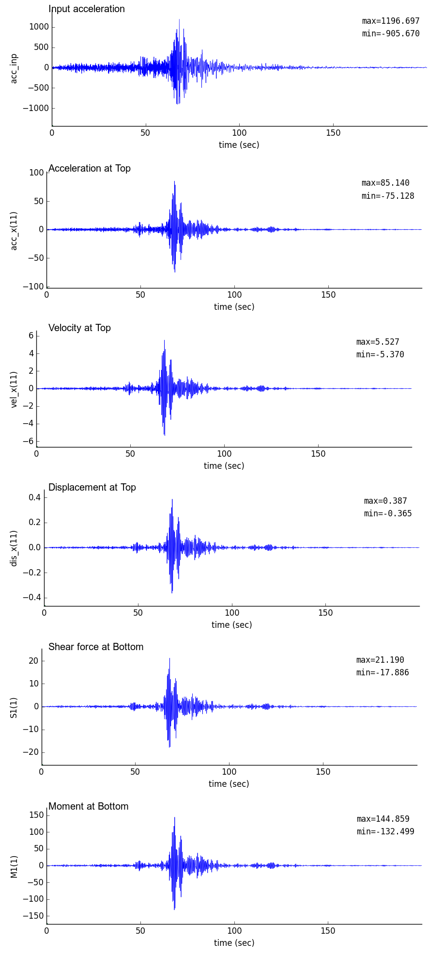 |
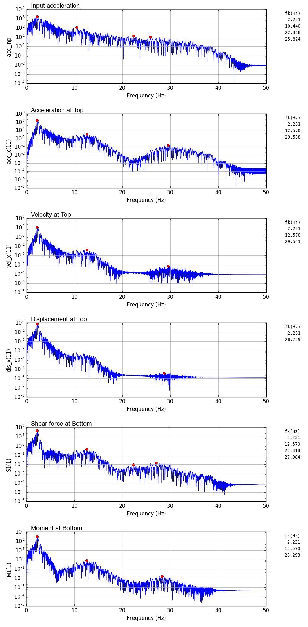 |
| Response time history (dt = 0.001 sec) | Fourier spectrum (dt = 0.001 sec) |
|---|
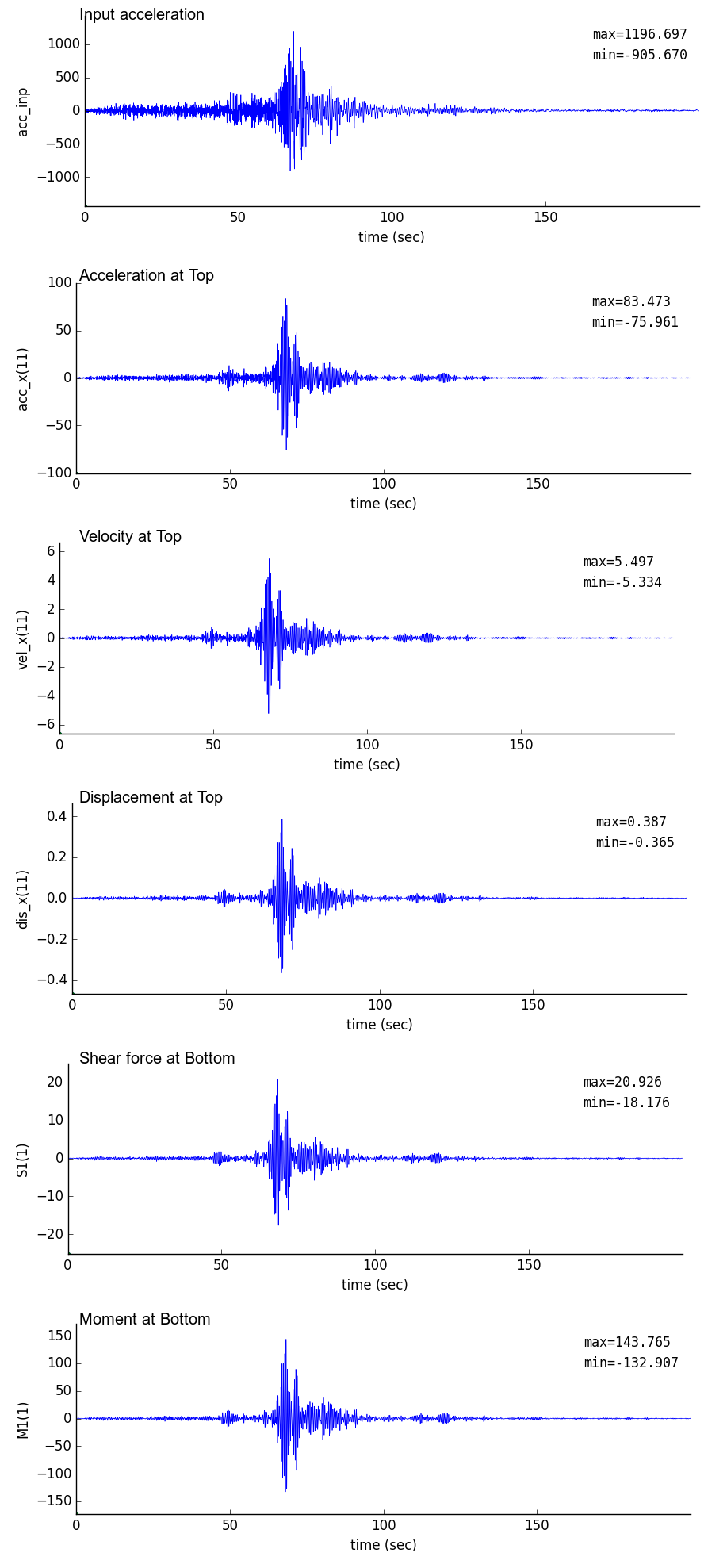 |
 |
2D Frame Geometrically Nonlinear Analysis
1. Outline
- This is a program for 2D frame geometrically nonlinear analysis. Large displacement of elastic frame members can be simulated, however it is assumed that an element follows small displacement theory.
- Beam element with 2 nodes is used. 1 node has 3 degrees of freedom in horizontal displacement, vertical displacement and rotation.
- Incremental Arc-Length Method is used to solve the incremental stiffness equation.
- Internal forces of the frame members are calculated using the linear stiffness matrix and the displacement without rigid rotation.
- Only nodal external force increment can be given as loads.
- In coordinate system, x-direction is defined as right-direction, y-direction is defined as upward direction and counterclockwise direction is defined as positive in rotation.
- Simultaneous linear equations are solved using numpy.linalg.solve(A, b).
- Input/Output file name can be defined arbitrarily with the format of space separater and those are inputted as command line arguments of a terminal.
| Valid boundary conditions |
|---|
| Item | Description |
|---|
| External force increment | Specify the loded nodes and load increment values |
| Forced displacement | Specify the nodes which are completely fixed. Only zero displacement can be allowed. |
2. FEM program
| Program name | Description |
|---|
| py_fem_gfrmAL.py | 2D Frame Geometrically Nonlinear Analysis program |
3. Command format for FEM analysis execution
python3 py_fem_gfrmAL.py inp.txt out.txt nnmax
| inp.txt | : Input data file (separated by space) |
| out.txt | : Output data file (separated by space) |
| nnmax | : Number of loading steps |
4. Input data format
npoin  nele  nsec  npfix  nlod  # Basic values for analysis
E  A  I                         # Material properties
    ..... (1 to nsec) .....     #
node_1  node_2  isec            # Element connectivity, material set number
    ..... (1 to nele) .....     #
x  y                            # Node coordinate of node
    ..... (1 to npoin) .....    #
lp  fix_x  fix_y  fix_r         # Restricted node number
    ..... (1 to npfix) .....    #
lp  df_x  df_y  df_r            # Loaded node and loading conditions (load increment)
    ..... (1 to nlod) .....     #     (omit data input if nlod=0)
| npoin, nele, nsec | : number of nodes, number of elements, number of material sets |
| npfix, nlod | : number of restricted nodes, number of loaded nodes |
| E, A, I | : elastic modulus, section area, moment of inertia |
| node_1, node_2, isec | : node-1, node-2, material set number |
| x, y | : x-coordinate, y-coordinate |
| lp, fix_x, fix_y, fix_r | : node, kind of restriction in x, y and rotation (0: free, 1: fixed) |
| lp, df_x, df_y, df_r | : loaded node, load increments in x, y and rotation |
5. Output data format
npoin  nele  nsec npfix  nlod  nnmax
    (Each value of above)
sec  E  A  I
    sec   : Material number
    E     : Elastic modulus
    A     : Section area
    I     : Moment of inertia
    ..... (1 to nsec) .....
node  x  y  fx  fy  fr  kox  koy  kor
    node   : Node number
    x      : x-coordinate
    y      : y-coordinate
    fx     : Load in x-direction
    fy     : Load in y-direction
    fr     : Moment load
    kox    : Index of restriction in x-direction (0: free, 1: fixed)
    koy    : Index of restriction in y-direction (0: free, 1: fixed)
    kor    : Index of restriction in rotation    (0: free, 1: fixed)
    ..... (1 to npoin) .....
elem  i  j  sec
    elem : Element number
    i    : Node number of start point
    j    : Node number of end point
    sec  : Material number
    ..... (1 to nele) .....
* nnn=0 iii=0 lam=0.0
node  fp-x  fp-y  fp-r  dis-x  dis-y  dis-r  dr-x  dr-y dr-r
    node  : Node number
    fp-x  : Total load in x-direction
    fp-y  : Total load in y-direction
    fp-r  : Total load in rotation
    dis-x : Displacement in x-direction
    dis-y : Displacement in y-direction
    dis-r : Displacement in rotation
    dr-x  : Un-balanced force in x-direction
    dr-y  : Un-balanced force in y-direction
    dr-r  : Un-balanced force in rotation
    ..... (1 to npoin) .....
elem  N_i  S_i  M_i  N_j  S_j  M_j
    elem : Element number
    N_i  : Axial force of node-i
    S_i  : Shear force of node-i
    M_i  : Moment of node-i
    N_j  : Axial force of node-j
    S_j  : Shear force of node-j
    M_j  : Moment of node-j
    ..... (1 to nele) .....
* nnn=1 iii=xx lam=xxx
node  fp-x  fp-y  fp-r  dis-x  dis-y  dis-r  dr-x  dr-y dr-r
    node  : Node number
    fp-x  : Total load in x-direction
    fp-y  : Total load in y-direction
    fp-r  : Total load in rotation
    dis-x : Displacement in x-direction
    dis-y : Displacement in y-direction
    dis-r : Displacement in rotation
    dr-x  : Un-balanced force in x-direction
    dr-y  : Un-balanced force in y-direction
    dr-r  : Un-balanced force in rotation
    ..... (1 to npoin) .....
elem  N_i  S_i  M_i  N_j  S_j  M_j
    elem : Element number
    N_i  : Axial force of node-i
    S_i  : Shear force of node-i
    M_i  : Moment of node-i
    N_j  : Axial force of node-j
    S_j  : Shear force of node-j
    M_j  : Moment of node-j
    ..... (1 to nele) .....

.... .... ....

* nnn=nnmax-1 iii=xx lam=xxx
node  fp-x  fp-y  fp-r  dis-x  dis-y  dis-r  dr-x  dr-y dr-r
    ..... (1 to npoin) .....
elem  N_i  S_i  M_i  N_j  S_j  M_j
    ..... (1 to nele) .....
n=(total degrees of freedom)  time=(calculation time)
| fp-x, fp-y, fp-r | : total loads in x, y-direction and rotation |
| dis-x, dis-y, dis-r | : total displacements in x, y-direction and rotation |
| dr-x, dr-y, dr-r | : unbalanced load in x, y-direction and rotation |
| N, S, M | : axial force, shearing force, moment |
| n | : Total degrees of freedom (the number of the variables) |
| time | : Calculation time |
6. Output sample
6.1 Input data and auxiliary program
6.2 Execution command for FEM analysis and drawing
# FEM calculation by Arc-Length method
python py_fem_gfrmAL.py inp_gfrm_canti.txt out_gfrm_canti.txt 70
python py_fem_gfrmAL.py inp_gfrm_cable.txt out_gfrm_cable.txt 290
python py_fem_gfrmAL.py inp_gfrm_arch.txt out_gfrm_arch.txt 310
python py_fem_gfrmAL.py inp_gfrm_lee.txt out_gfrm_lee.txt 160

# Drawing of Load-displacement curve
python py_fig_gfrm.py out_gfrm_canti.txt 11 11 -411.07 1000 1000 \$u/L\$ $\v/L\$ \$u/L\$\,$\v/L\$ \$P/P_{cr}\$ LL
python py_fig_gfrm.py out_gfrm_cable.txt 12 11 -1644.3 1000 1000 \$u/L\$ \$v/L\$ \$u/L\$\,\$v/L\$ \$P/P_{cr}\$ LL
python py_fig_gfrm.py out_gfrm_arch.txt 21 21 -666.4 -500 -500 \$u/R\$ \$v/R\$ \$u/R\$\,\$v/R\$ \$P\\cdot\(R^2/EI\)\$ UL
python py_fig_gfrm.py out_gfrm_lee.txt 13 13 -166.6 1000 -1000 \$u/L\$ \$v/L\$ \$u/L\$\,\$v/L\$ \$P\\cdot\(L^2/EI\)\$ LL

# Drawing of displacement mode
python py_fig_gfrm_mode.py
Execution command for load-displacement cutve drawing
python py_fig_gfrm.py out.txt node-L node-D nd-L nd-u nd-v leg-u leg-v x-Label y-Label loc
| out.txt | : FEM output data (separated by space) |
| node-L | : node for load-axis |
| node-D | : node for displacement axis |
| nd-L | : coefficient for dimensionless load (including sign) |
| nd-u | : coefficient for dimensionless displacement in x-direction (uncluding sign) |
| nd-v | : coefficient for dimensionless displacement in y-direction (uncluding sign) |
| leg-u | : label of displacement in x-direction for legend |
| leg-v | : label of displacement in y-direction for legend |
| x-Label | : label of x-axis (displacement) |
| y-Label | : label of y-axis (load) |
| loc | : location of legend |
6.3 Sample drawing
| Vertical cantilever under axial compression (inp_gfrm_canti.txt) |
|---|
L=1,000mm, E=200,000MPa, A=100m$^2$, I=833m$^4$
Initial deflection $v_0$=1mm
Buckling load $P_{cr}=\pi^2 EI / 4 L^2$=411.07N |
| Displacement mode | Displacements at Top |
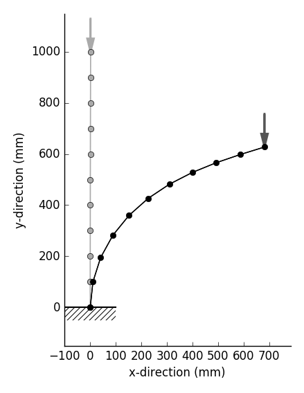 |
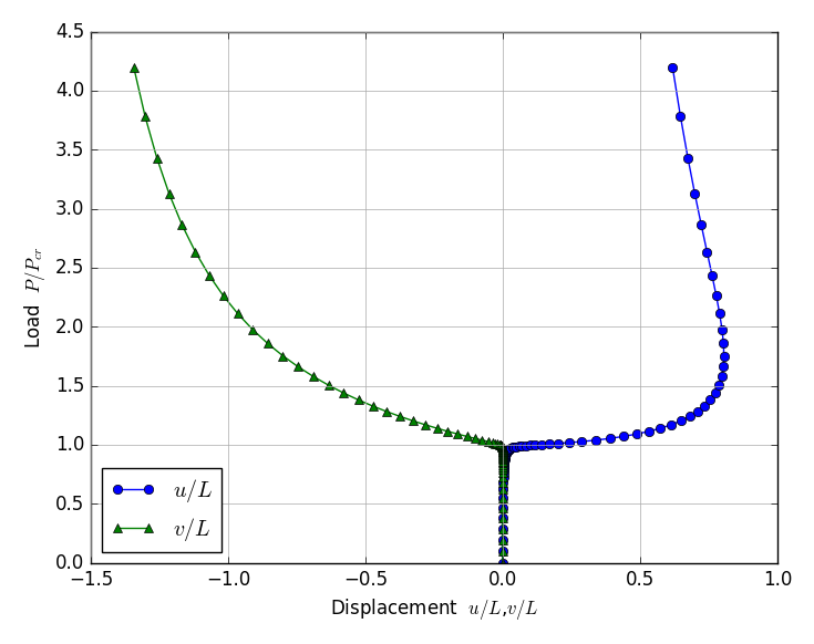 |
| Vertical cantilever with tensile cable (inp_gfrm_cable.txt) |
|---|
Column: L=1,000mm, E=200,000MPa, A=100m$^2$, I=833m$^4$
Cable: L=1,000mm, E=200,000MPa, A=28.3$^2$
Initial deflection $v_0$=5mm
Buckling load $P_{cr}=\pi^2 EI / L^2$=1644.3NN |
| Displacement mode | Displacements at Top |
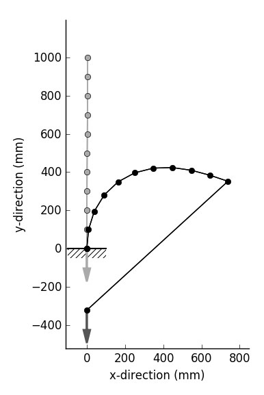 |
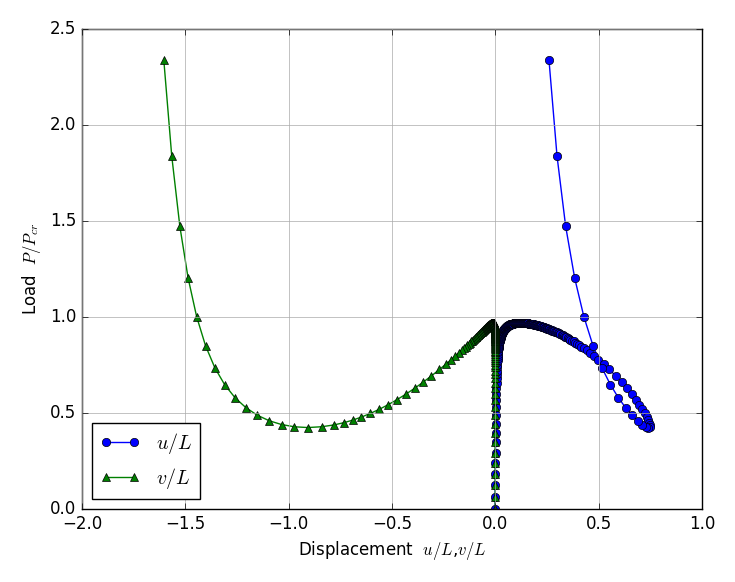 |
| Arch under the vertical concentrated load with asymmetrcal supports (inp_gfrm_arch.txt) |
|---|
| R=500mm, Center angle=215$^\circ$, E=200,000MPa, A=100m$^2$, I=833m$^4$ |
| Displacement mode | Displacements at Loading point |
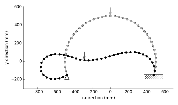 |
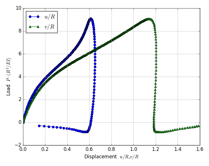 |
| Frame under the vertical concentrated load (inp_gfrm_lee.txt) |
|---|
| L=1000mm, E=200,000MPa, A=100m$^2$, I=833m$^4$ |
| Displacement mode | Displacements at Loading point |
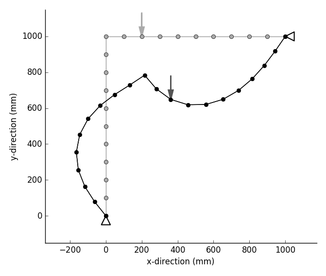 |
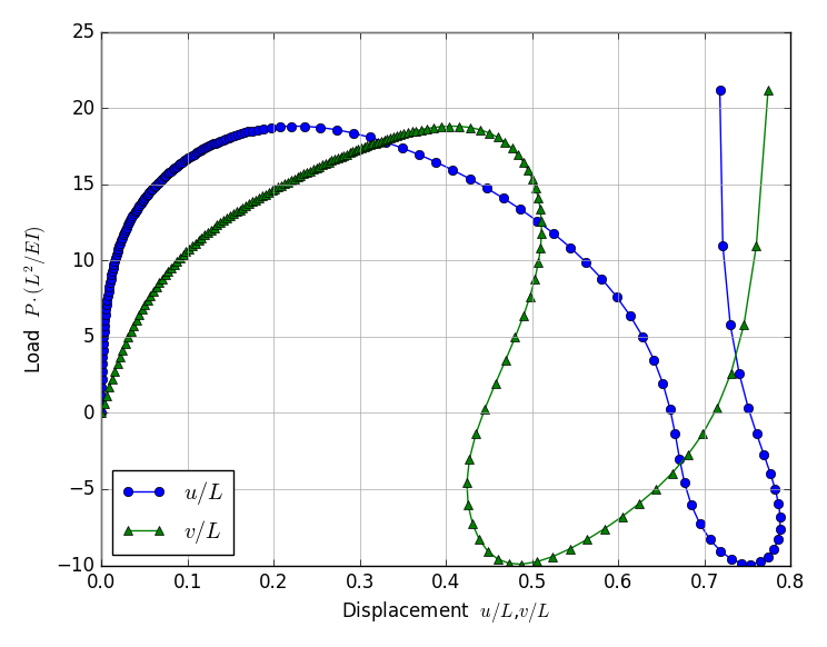 |
2D Frame Buckling Analysis
1. Outline
- This is a program for 2D elastic frame linear backling analysis. To calculate backling load, engenvalue analysis is used.
- Beam element with 2 nodes is used. 1 node has 3 degrees of freedom in horizontal displacement, vertical displacement and rotation.
- In coordinate system, x-direction is defined as right-direction, y-direction is defined as upward direction and counterclockwise direction is defined as positive in rotation.
- Characteristic equation are solved using w,vr=scipy.linalg.eig(K, M) as a generalized eigenvalue problem
- Regarding the axila force for eigenvalue analisys, compressive force shall have positive sign.
- Before eigenvalue analysis, linear analysis shall be carried out using initial load input, because it is necessary to define the initial axial force for eigenvalue analysis.
- Since above step is required for buckling analysis, buckling load is estimated as a product of eigenvalue and initial load.
- Simultaneous linear equations for initial analysis are solved using numpy.linalg.solve(A, b).
- Input/Output file name can be defined arbitrarily with the format of space separater and those are inputted as command line arguments of a terminal.
| Valid boundary conditions |
|---|
| Item | Description |
|---|
| External force increment | Specify the loded nodes and unit load values |
| Forced displacement | Specify the nodes which are completely fixed. Only zero displacement can be allowed. |
2. FEM program
| Program name | Description |
|---|
| py_fem_bfrm.py | 2D Frame Buckling Analysis program |
3. Command format for FEM analysis execution
python3 py_fem_bfrm.py inp.txt out.txt
| inp.txt | : Input data file (separated by space) |
| out.txt | : Output data file (separated by space) |
4. Input data format
npoin  nele  nsec  npfix  nlod  # Basic values for analysis
E  A  I                         # Material properties
    ..... (1 to nsec) .....     #
node_1  node_2  isec            # Element connectivity, material set number
    ..... (1 to nele) .....     #
x  y                            # Node coordinate of node
    ..... (1 to npoin) .....    #
lp  fix_x  fix_y  fix_r         # Restricted node number
    ..... (1 to npfix) .....    #
lp  df_x  df_y  df_r            # Loaded node and loading conditions
    ..... (1 to nlod) .....     #     (omit data input if nlod=0)
| npoin, nele, nsec | : number of nodes, number of elements, number of material sets |
| npfix, nlod | : number of restricted nodes, number of loaded nodes |
| E, A, I | : elastic modulus, section area, moment of inertia |
| node_1, node_2, isec | : node-1, node-2, material set number |
| x, y | : x-coordinate, y-coordinate |
| lp, fix_x, fix_y, fix_r | : node, kind of restriction in x, y and rotation (0: free, 1: fixed) |
| lp, df_x, df_y, df_r | : loaded node, unit loads in x, y and rotation |
5. Output data format
npoin  nele  nsec npfix  nlod
    (Each value of above)
sec  E  A  I
    sec   : Material number
    E     : Elastic modulus
    A     : Section area
    I     : Moment of inertia
    ..... (1 to nsec) .....
node  x  y  fx  fy  fr  kox  koy  kor
    node   : Node number
    x      : x-coordinate
    y      : y-coordinate
    fx     : Load in x-direction
    fy     : Load in y-direction
    fr     : Moment load
    kox    : Index of restriction in x-direction (0: free, 1: fixed)
    koy    : Index of restriction in y-direction (0: free, 1: fixed)
    kor    : Index of restriction in rotation    (0: free, 1: fixed)
    ..... (1 to npoin) .....
elem  i  j  sec
    elem : Element number
    i    : Node number of start point
    j    : Node number of end point
    sec  : Material number
    ..... (1 to nele) .....
Order         1       2       3  ......
lambda     w[1]   w[2]    w[3]  ......
v[  1]   v[1,1]  v[1,2]  v[1,3]  ......
v[  2]   v[1,1]  v[1,2]  v[1,3]  ......
......   ......  ......  ......  ......
v[  n]   v[1,1]  v[1,2]  v[1,3]  ......
    Order   : Ranking
    w[i]    : Buckling coefficient (eigen value)
    v[j,i]  : Element of eigen vector
n=(total degrees of freedom)  time=(calculation time)
| fx, fy, fr | : initial loads in x, y-direction and rotation |
| w[i] | : eigenvalue (ascending order) |
| v[j,i] | : eigen vector (displacement mode) |
| n | : Total degrees of freedom (the number of the variables) |
| time | : Calculation time |
6. Output sample
Input data sample and auxiliary program
6.2 Execution command for FEM analysis and drawing
After execution of eigenvalue analysis and drawing program, combination image file is created using ImageMagick 'convert' command.
python py_fem_bfrm.py inp_circ.txt out_circ.txt
python py_fig_bfrm_mode.py out_circ.txt

convert +append fig_0.png fig_1.png fig_2.png _1.png
convert +append fig_3.png fig_4.png fig_5.png _2.png
convert +append fig_6.png fig_7.png fig_8.png _3.png
convert +append fig_9.png fig_10.png fig_11.png _4.png
convert -append _1.png _2.png _3.png _4.png fig_bmode.png
6.3 Sample drawing
Conditions
Diameter of the circular ring: 3,000mm, material thickness: 20mm, materithickness: 20mm, depth: 1mm
Elastic modulus: 200,000MPa, Initial external water pressure: 1MPa
Number of nodes: 180, number of elements: 180
Theoritical buckling pressure of circular ring
Buckling pressure of circular ring can be calculated as follow, under the condition that 'the direction of external force is not changed after buckling'.
\begin{equation}
P_{cr}=\cfrac{n^2 E I}{R^3} \qquad (n=2, 3, 4, ......)
\end{equation}
The conditions for calculation is that E=200,000MPa, I=666.666mm$^4$, R=1500mm.
Comparison of buckling pressure between the theoritical value and eigenvalue analysis result
| Mode (n) | 2 | 3 | 4 | 5 | 6 | 7 | 8 |
|---|
| Theoritical value (MPa) | 0.158 | 0.356 | 0.632 | 0.988 | 1.422 | 1.936 | 2.528 |
|---|
| Eigenvalue analysis (MPa) | 0.158 | 0.356
0.356 | 0.627
0.632 | 0.988
0.988 | 1.413
1.423 | 1.936
1.936 | 2.528 |
|---|
| Buckling displacement mode of circular ring under the external water pressure |
|---|
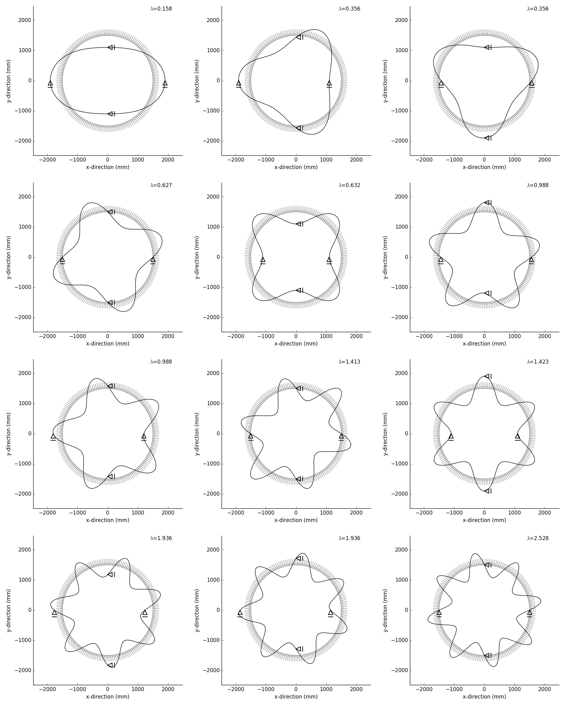 |
1D Thermal Conductivity Analysis
1. Outline
- This is a program for 1D unsteady thermal conductivity analysis. This program can not treat steady problem.
- As boundary conditions, thermal insulation boundary and heat transfer boundary can be considered.
- Heating material such as cement concretecan also be used .
- This program can considere the some lift placing of concrete by specifying the placing time and available element at the time.
- 2 node linear element is used. 1 node has 1 degree of freedom of temperature or heat flux.
- In coordinate system, x-direction is defined as vertical upward direction.
- Crank-Nicolson method is used for the discretization of the time.
- Simultaneous linear equations are solved using numpy.linalg.inv(A).
Although this solving process has repeating process for time history analysis, matrix for calculation is not changed if the time increment is not changed.
Therefore, to calculate an inverse matrix is carried out only one time, and it is used to calculate the time history of the temperature until the end of the calculation time.
- Input/Output file name can be defined arbitrarily with the format of space separater and those are inputted as command line arguments of a terminal.
In addition, it is necessary to prepare the input file for time history of outside temperatures of heat transfer boundary.
| Valid boundary conditions |
|---|
| Item | Description |
|---|
| Thermal insulation boundary | No input means thermal insulation boundary |
| Heat transfer boundary | Specify the sides of element, heat transfer coefficient and time history of temperature at outside |
About temperature given boundary
This program can not treat temperature given boundary. Although the treatment of temperature given boundary condition has been tried, only unexpected results have been obtained. However, if large heat transfer rate is used for heat transfer boundary, it is possible to simulate almost the same condition as temperature given boundary.
2. FEM program
| Program name | Description |
|---|
| py_fem_1Dheat.py | 1D Thermal Conductivity Analysis program |
3. Command format for FEM analysis execution
python py_fem_1Dheat.py inp1.txt inp2.txt out.txt
| inp1.txt | : First input data file for analysis model (separated by space) |
| inp2.txt | : Second input data file for time histories of outside temperature of heat transfer boundary (separated by space) |
| out.txt | : Output data file (separated by space) |
4. Input data format
(1) Analysis model data
npoin  nele  nsec  koB  koT  delta  nlift  # Basic values for analysis
Ak  Ac  Arho  Tk  Al  AA                   # Material properties
     ..... (1 to nsec) .....               #
tlift_1  tlift_2  .... (1 line input) .... # Placing time of each lift
alphac_B  alphac_T                         # Heat transfer rates of bottom and top
node-1  node-2  isec  lift                 # Element connectivity, Material set number, lift number
     ..... (1 to nele) .....               #   (counterclockwise order of node numbers)
x  T0                                      # Coordinates of node, initial temperature of node
     ..... (1 to npoin) .....              #
n1out                                 # Number of nodes for output of temperature time history
n1node_1  ..... (1 line input) .....  # Node number for above
n2out                                 # frequency of output of temperatures of all nodes
n2step_1  ..... (1 line input) .....  # Time step number for above (Omit data input if ntout=0)
| npoin, nele, nsec | : number of nodes, number of elements, number of material sets |
| koB | : Bottom end boundary condition (0: thermal insulation, 1: heat transfer boundary) |
| koT | : Top end boundary condition (0: thermal insulation, 1: heat transfer boundary) |
| delta | : time increment |
| nlift | : number of lifts |
| Ak, Ac, Arho | : heat conductivity coefficient, specific heat, unit weight |
| Tk, Al | : maximum temperature rise, coefficient of heat release rate (for heating material) |
| AA | : section area of element |
| x, T0 | : x coordinate, initial temperature of node |
| n1out | : number of nodes for all time history output |
| n1node | : node numbers for all time history output |
| n2out | : number of steps for all nodes temperature output |
| n2step | : step numbers for all nodes temperature output |
(2) Time history data of outside of heat transfer boundary
To input 3 columns values are required. Even if the boundary condition is not heat transfer, the column shall be filled by zero.
 0   TcinB[0]  TcinT[0]
 1   TcinB[1]  TcinT[1]
 2   TcinB[2]  TcinT[2]
 ..  ........  ........
 i   TcinB[i]  TcinT[i]
 ..  ........  ........
 .... (until end of calculation time) ....
| TcinB | : outside temperature for bottom end heat transfer boundary |
| TcinT | : outside temperature for top end heat transfer boundary |
5. Output data format
npoin  nele  nsec  koB  koT  delta  nlift  niii  n1out  n2out
    (Each value of above)
sec  Ak  Ac  Arho  Tk  Al  AA
    sec  : Material number
    Ak   : Heat conductivity coefficient
    Ac   : Specific heat
    Arho : Unit weight
    Tk   : Maximum temperature rize
    Al   : Heat release rate
    AA   : Section area of element
    ..... (1 to nsec) .....
node  x  tempe0  alphac
    node   : Node number
    x      : x-ccordinate
    tempe0 : Initial temperature
    alphac : Heat transfer rate of bottom and top node
    ..... (1 to npoin) .....
elem  i  j  sec  lift  time
    elem : Element number
    i    : Node number of start point
    j    : Node number of second point
    sec  : Material number
    lift : Lift number
    time : Placing time of lift
    ..... (1 to nele) .....
iii  ttime  Node_(xx)  Node_(xx)  Node_(xx) .....
    iii       : Time step
    ttime     : Time
    Node-(xx) : Node number
    Time historis of each node temperature are written.
    ..... (0 to end of calculation time) .....
node  t=0.0  t=(xx)  t=(xx)0  t=(xx) .....
    node   : Node number
    t=(xx) : Specified time
    Node temperatures at specified time are written.
    ..... (1 to npoin) .....
n=(total degrees of freedom)  time=(calculation time)
6. Output sample
6.1 Input data and auxiliary program
6.2 Outline of sample analysis model
Model considered are that new concrete 5 lifts with height of 2m for each lift are placed on old existing concrete with thickness of 10m.
| Characteristics of model |
|---|
| Heat conductivity coefficient | 2.5 kcal/m h $^{\circ}$C |
| Specific heat | 0.28 kcal/kg $^{\circ}$C |
| Unit weight | 2350 kg/m$^3$ |
Adiabatic temperature raise
for new concrete | $T=K\cdot(1-e^{-\alpha t})$, K=40$^{\circ}$C, α=0.2, t: hour |
| Element section area | 1m$^2$ |
| Model | Total length: 20m
Old concrete: 10m
New concrete: 10m,
5 lifts with height of 2m, Placing interval: 3 days (72 hours) |
| Conditions for analysis |
|---|
| New concrete placing temperature | 30 $^{\circ}$C |
| Old concrete initial temperature | from 10 $^{\circ}$C at bottom to 20 $^{\circ}$C at surface |
| Boundary condition of bottom | Temperature fixed with outside temperature 10 $^{\circ}$c (approximately)
Heat transfer rate of bottom boundary: 10000 kcal/m$^2$ h $^{\circ}$C
|
| Boundary condition of top | Heat transfer boundary with outside temperature of 20 $^{\circ}$C
Heat transfer rate of top boundary: 10 kcal/m$^2$ h $^{\circ}$C |
| Time increment for analysis | 0.1 hour |
6.3 Execution command for FEM analysis and drawing
python py_fem_1Dheat.py inp_100L1.txt inp_2L2.txt out_100L.txt
python py_fem_1Dheat.py inp_40L1.txt inp_2L2.txt out_40L.txt
python py_fem_1Dheat.py inp_20L1.txt inp_2L2.txt out_20L.txt

python py_fig_1Dheat.py out_100L.txt
cp _fig_tem_his.png fig_his_100.png

python py_fig_1Dheat.py out_40L.txt
cp _fig_tem_his.png fig_his_040.png

python py_fig_1Dheat.py out_20L.txt
cp _fig_tem_his.png fig_his_020.png
| inp_100L1.txt | : FEM analysis model input data file (100 elements) |
| inp_40L1.txt | : FEM analysis model input data file (40 elements) |
| inp_20L1.txt | : FEM analysis model input data file (20 elements) |
| inp_2L2.txt | : FEM outside temperature time history input data file |
| out_1D.txt | : FEM analysis output data file |
Program 'py_fig_1Dheat.py' creates a image file named '_fig_tem_his.png' automatically.
6.4 Sample drawing
png images created by program 'py_fig_1Dheat.py' are shown below.
The 3 cases of element division (20, 40, 100) are considered.
Something is wrong in the case of 20 elements. When parts surrounded with red ovals are payed attention, followings can be founded.
- Even though concrete placing temperature is 30 $^{\circ}$C and maximum temperature rise of concrete is 40 $^{\circ}$C, the maximum concrete temperature after placing is greater than 75 $^{\circ}$C.
- In the old concrete near the boundary of new concrete, unbelievable temperature time history can be observed.
Above phenomenon is improved as number of elements increases.
| 20 elements model |
|---|
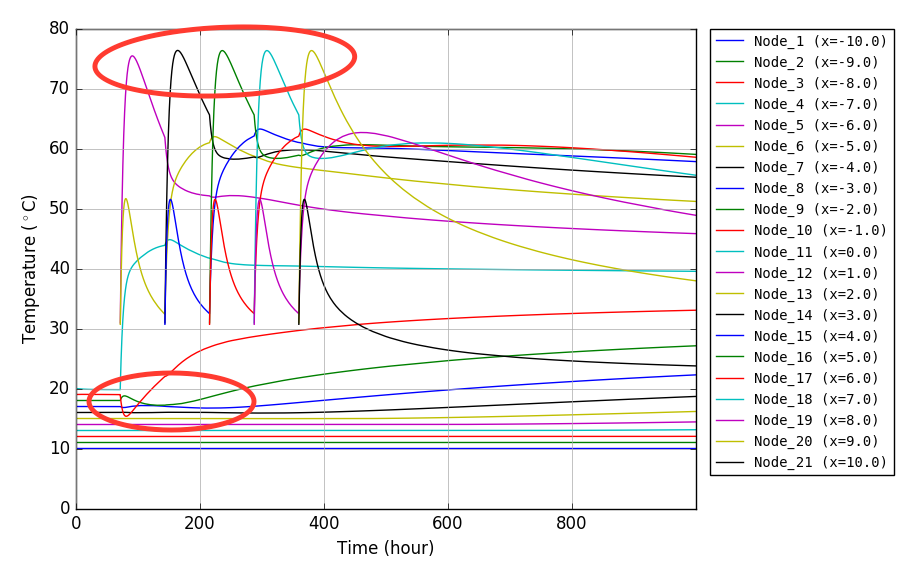 |
| 40 elements model |
|---|
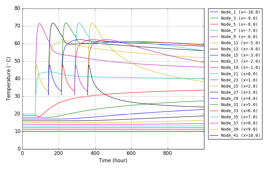 |
| 100 elements model |
|---|
 |